Project 1: Images of the Russian Empire: Colorizing the Prokudin-Gorskii Photo Collection
Overview
Prokudin-Gorskii recorded each scene through blue, green, and red filters in three separate exposures on a glass plate. The digitized scan contains those grayscale exposures stacked vertically in BGR order. Each exposure records how much light passed through its filter. Together, they provide the blue, green, and red values needed to reconstruct a color photograph.
I load each scan and convert its unsigned integer pixel values to floats between 0 and 1. I divide the scan’s height by three and extract three equal-height arrays. Simply stacking these arrays produces colored outlines around objects because the separate exposures are displaced. I use the blue exposure as a fixed reference and find separate horizontal and vertical shifts for green and red. After applying those shifts, I stack the arrays in RGB order to form the color image.
Normalized Cross-Correlation (NCC)
I use normalized cross-correlation (NCC) to score how closely the blue channel matches a shifted green or red channel. Let A and B be the two arrays of interior pixels used for comparison. I subtract each array’s mean to get centered arrays a = A − mean(A) and b = B − mean(B). I then calculate:
The index i runs over corresponding pixel positions in the two arrays. The numerator is their dot product: I multiply each pair of centered pixel values and add the products. The denominator is the product of their Euclidean lengths. Dividing by it normalizes the score, which ranges from −1 to 1 for nonconstant arrays. A score near 1 means the intensity patterns match closely. I select the shift with the highest score.
Mean subtraction and normalization help NCC compare channels with different overall brightness and contrast. Individual objects can still look different across channels, which can cause a poor match.
I calculate NCC on the central regions selected by the alignment function. If either centered array has zero length, I return a score of negative infinity to avoid division by zero and prevent that candidate from winning.
Single-Scale Alignment
Single-scale alignment searches at the original image resolution. I keep blue fixed and search separately for the best green and red shifts. For each channel, I use two loops to test every row and column shift from −15 to +15 pixels, including both endpoints. This gives 31 × 31 = 961 candidate shifts per channel.
For each candidate, I shift the entire moving channel with NumPy’s roll operation and calculate NCC against blue. I exclude a margin around each image and calculate NCC only on the remaining central region. This keeps the scan’s black and white borders from affecting the score. I compare the same central pixel positions for every candidate shift. The interior margin also excludes pixels that roll moves from one edge to the opposite edge.
I keep the candidate with the highest NCC score and return its shift. All offsets below are in (row, column) order: a positive row value moves the channel down, and a positive column value moves it right. For Cathedral, the selected green shift is (5, 2), so I move green 5 pixels down and 2 pixels right. Red is shifted independently by (12, 3).
I apply the selected shifts to the original green and red arrays, then stack red, green, and the fixed blue array in RGB order.
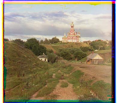
Green: (5, 2)
Red: (12, 3)
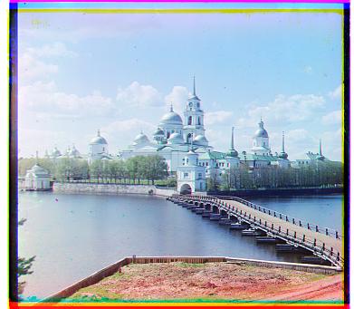
Green: (-3, 2)
Red: (3, 2)
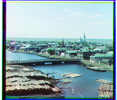
Green: (3, 3)
Red: (6, 3)
Pyramid Alignment
The TIFF scans are much larger than the JPEGs, so their channel displacements can exceed the single-scale search window. Increasing that window at full resolution would require more candidate shifts, each with an NCC calculation over millions of pixels. An image pyramid lets me estimate large shifts on smaller images before refining them at full resolution.
I build a separate pyramid for each channel, starting with the original array. I repeatedly resize the most recent level to half its width and height until its longest side is at most 200 pixels. The resizing applies anti-aliasing, which smooths fine details before downsampling so they do not produce false patterns in the smaller image. I store the levels in a list from largest to smallest.
Alignment goes through that list in reverse order, from smallest to largest. I first search ±15 pixels in both directions around (0, 0) at the smallest level. The single-scale search calculates NCC on the two channels’ central regions and returns the highest-scoring shift. I perform this process separately for green against blue and red against blue.
At each larger level, I double both components of the previous shift because the image dimensions approximately double. A shift of (3, 5) becomes an initial estimate of (6, 10). I then search ±2 pixels around that estimate: rows 4 through 8 and columns 8 through 12 in this example. This tests 25 candidates and corrects small errors from downsampling and rounding. The search returns the full shift at that level, which becomes the estimate for the next level.
I repeat this refinement until I reach the original resolution. I apply the final shifts to the original green and red arrays and combine them with blue in RGB order, so the saved image retains the original channel dimensions. I use the same 200-pixel size limit, ±15 initial window, and ±2 refinement window for all 17 supplied and additional scans.
Pyramid Results for Given Images
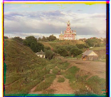
Green: (5, 2)
Red: (12, 3)
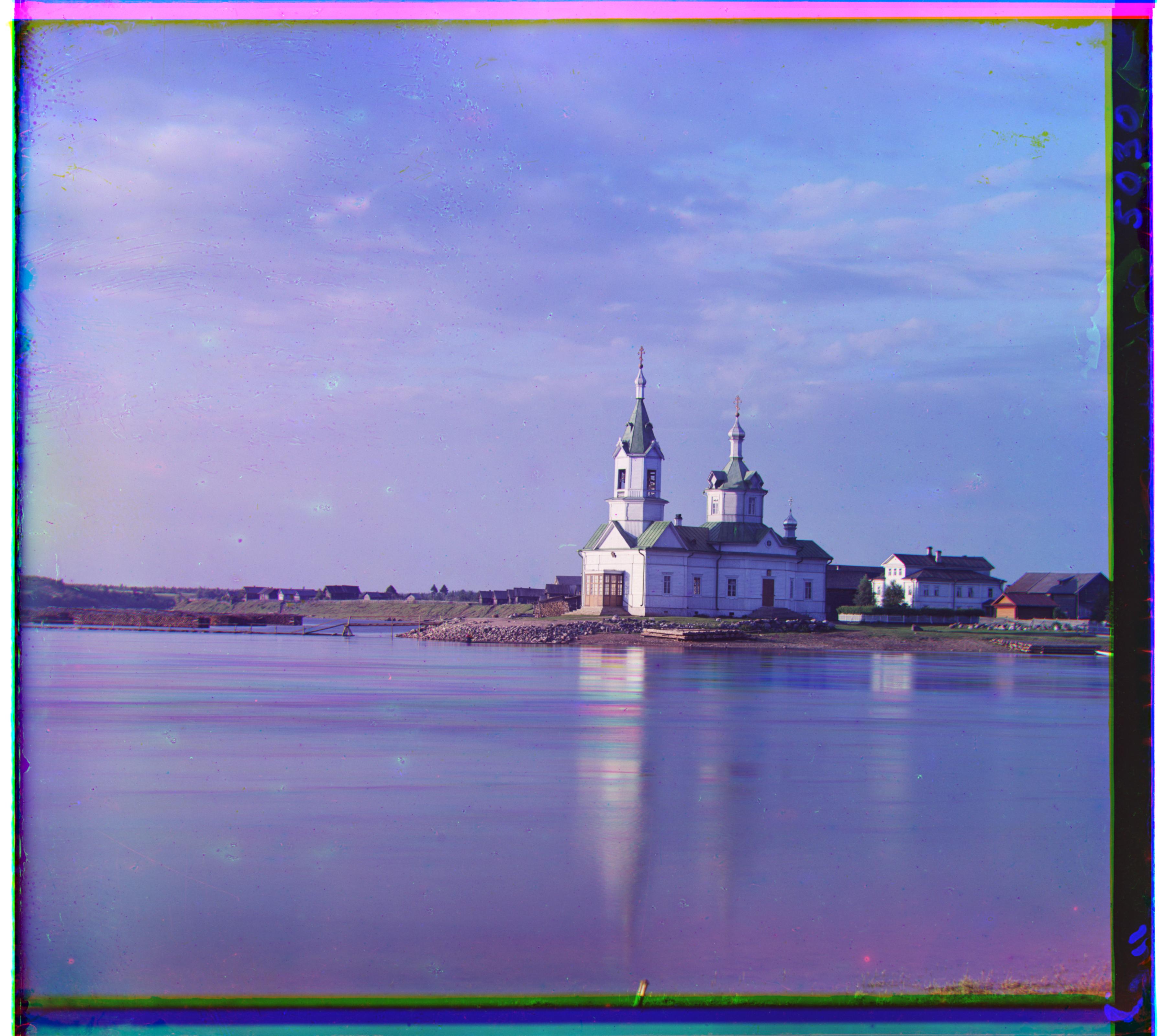
Green: (25, 4)
Red: (58, -4)
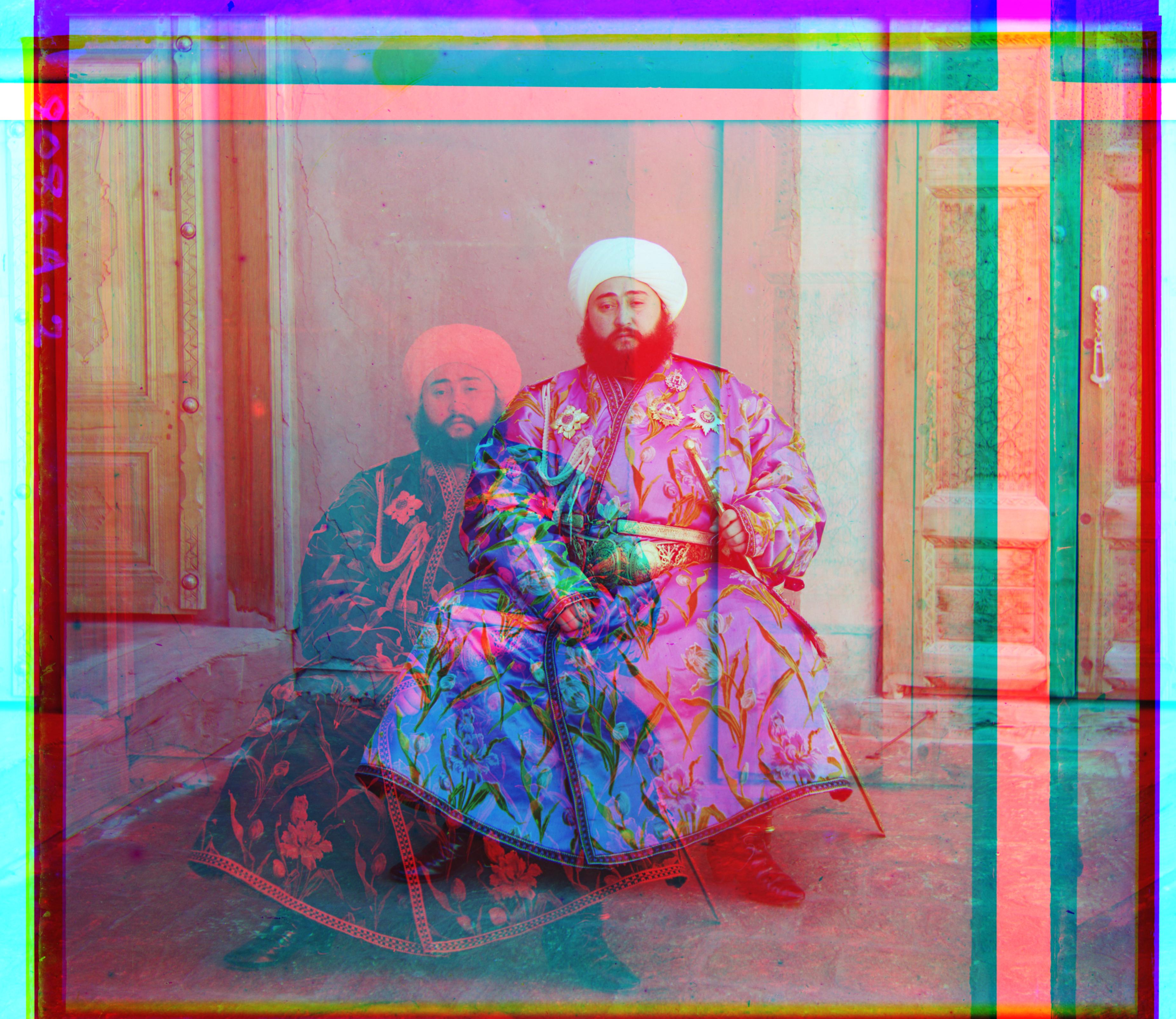
Green: (49, 24)
Red: (378, -481)
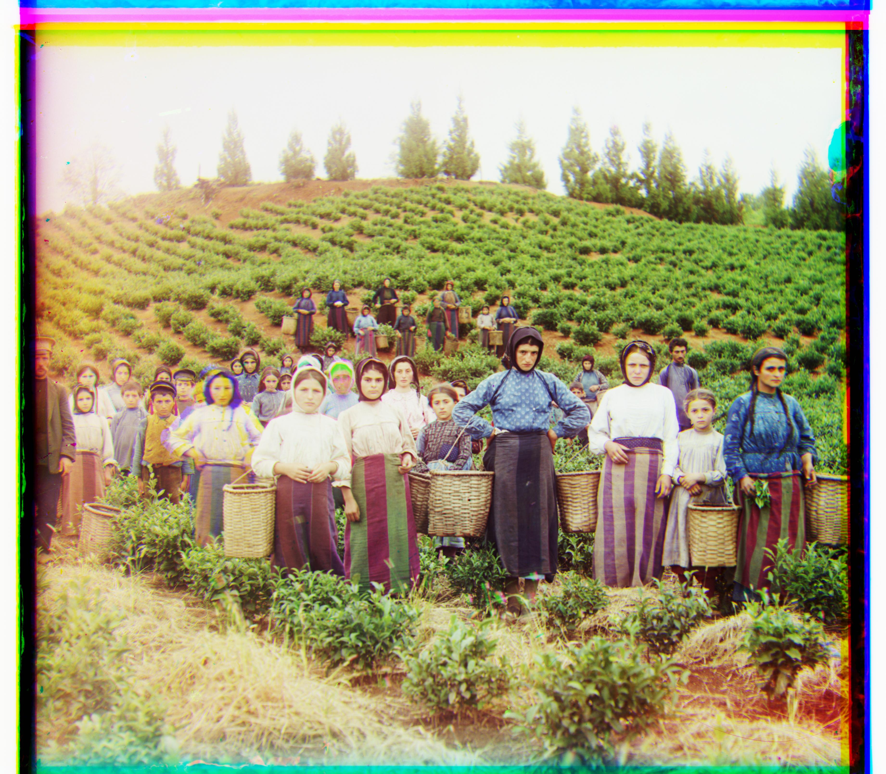
Green: (60, 17)
Red: (124, 13)
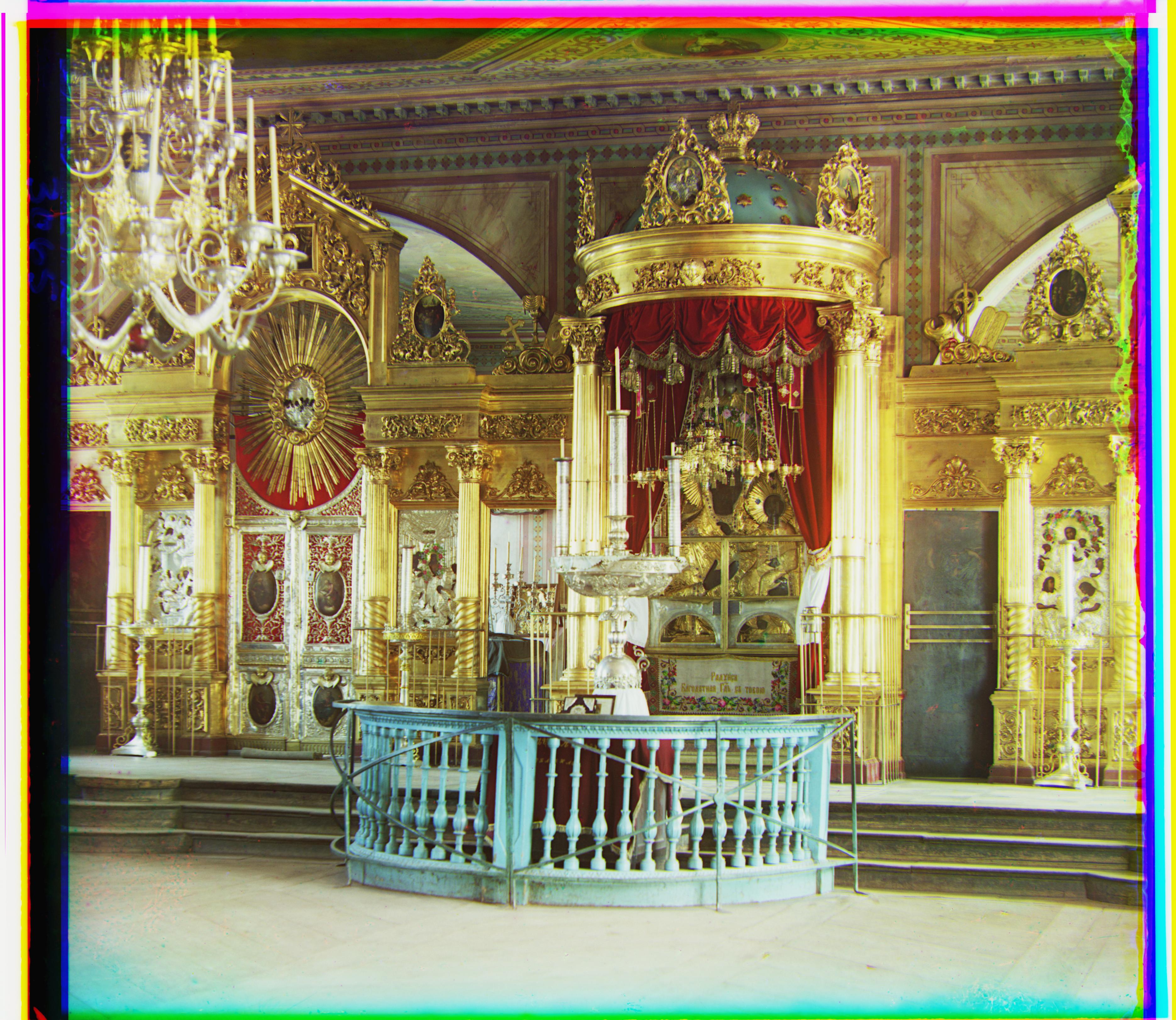
Green: (41, 17)
Red: (89, 23)
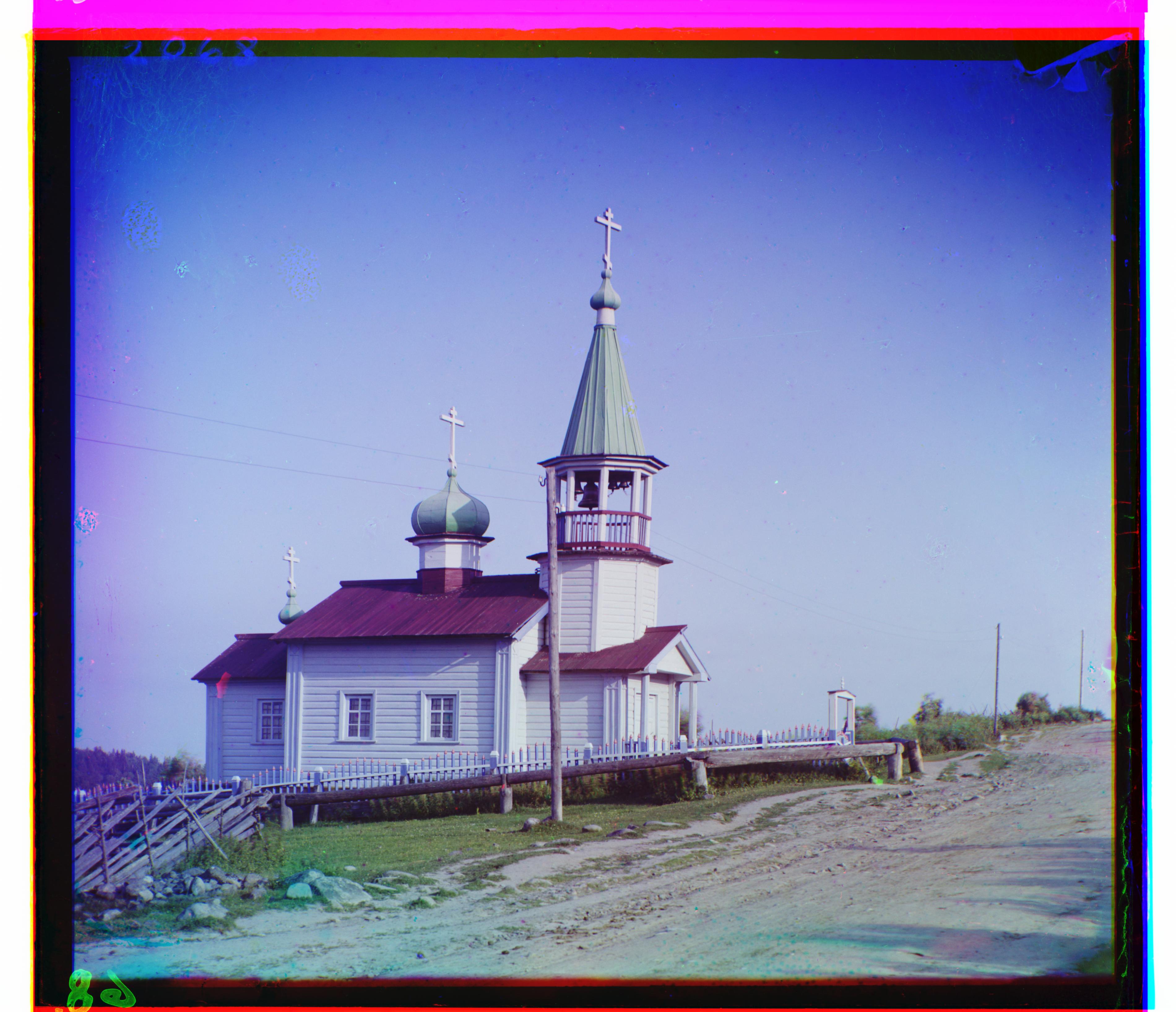
Green: (40, 7)
Red: (130, 11)
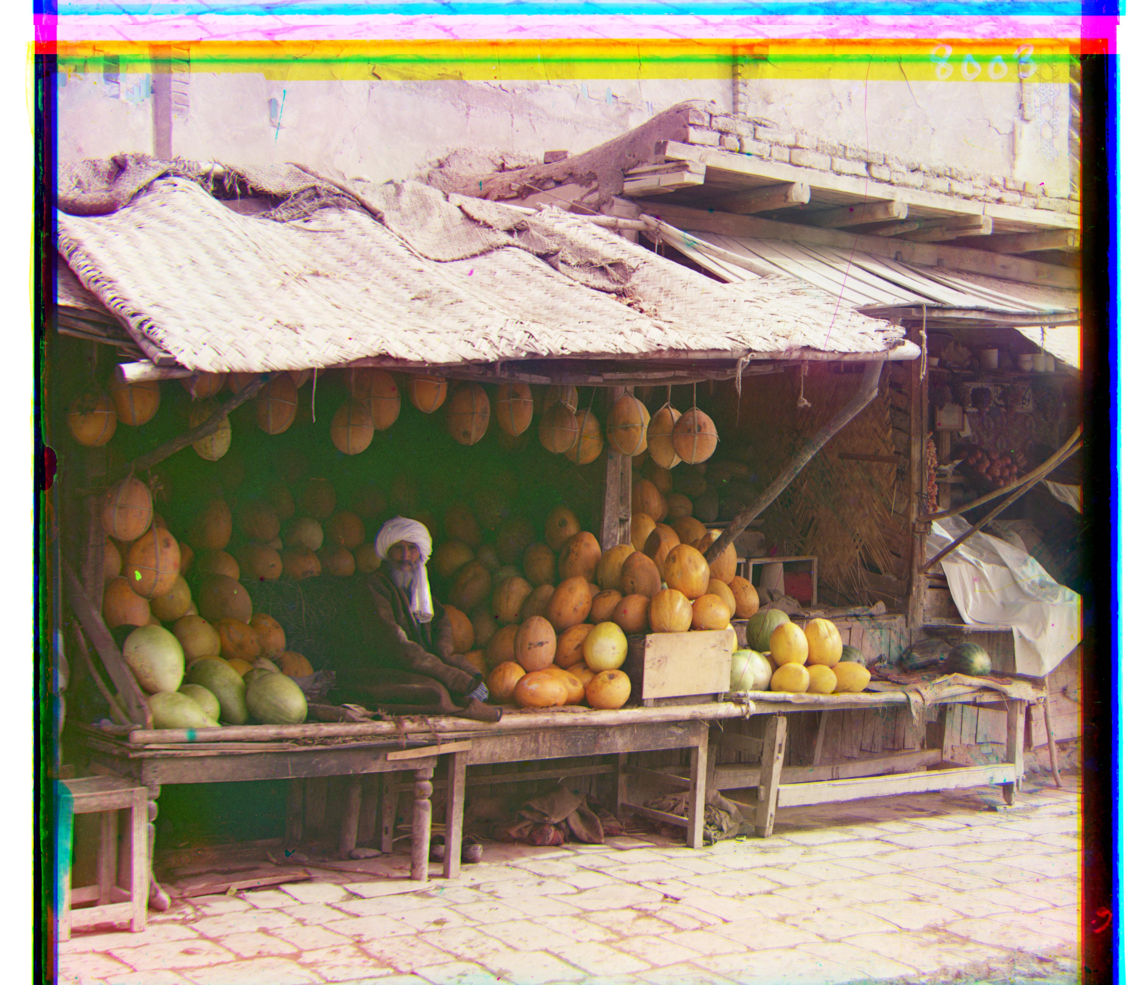
Green: (82, 11)
Red: (178, 13)
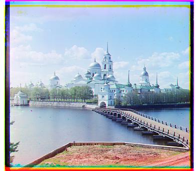
Green: (-3, 2)
Red: (3, 2)
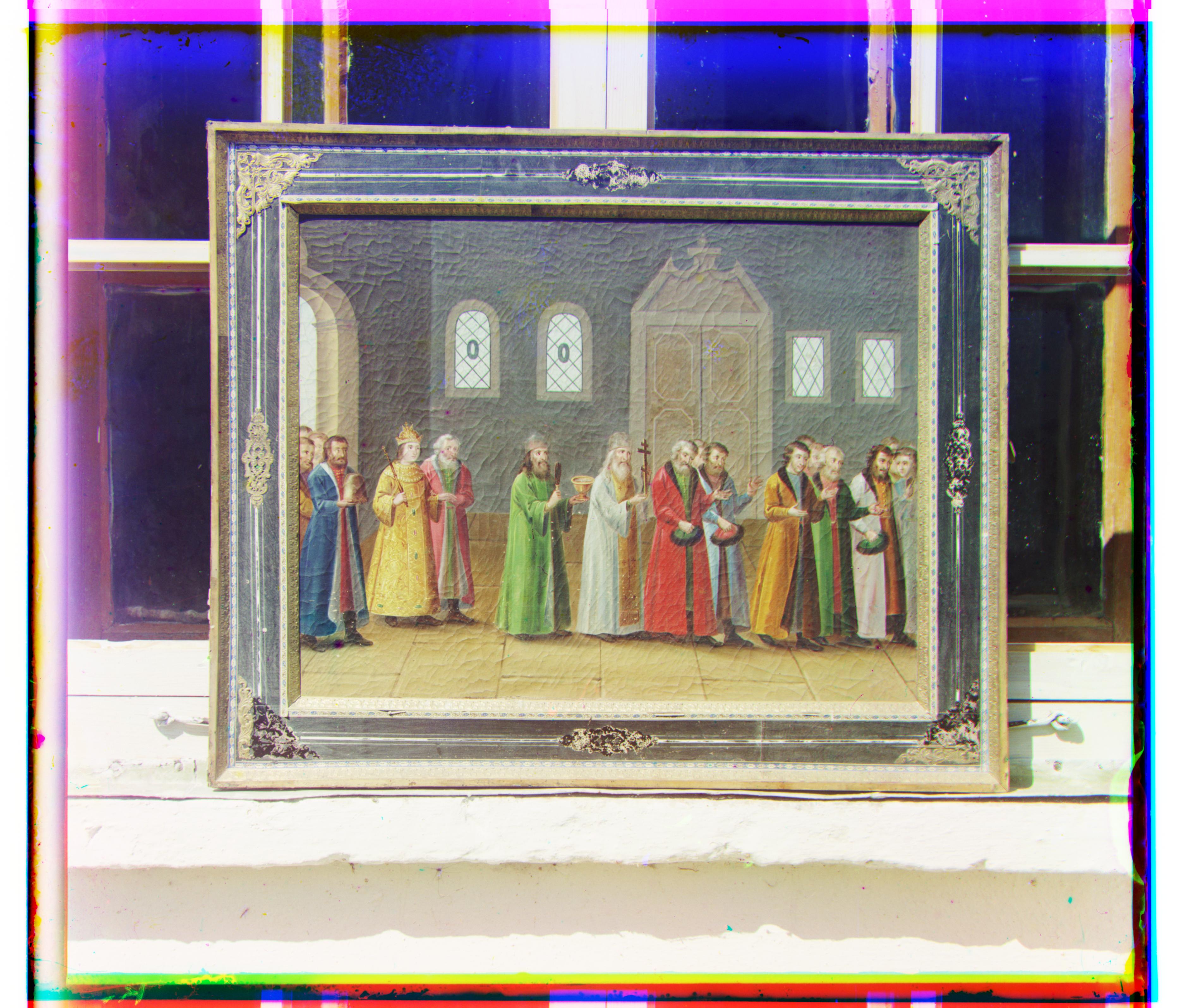
Green: (28, 3)
Red: (68, 7)
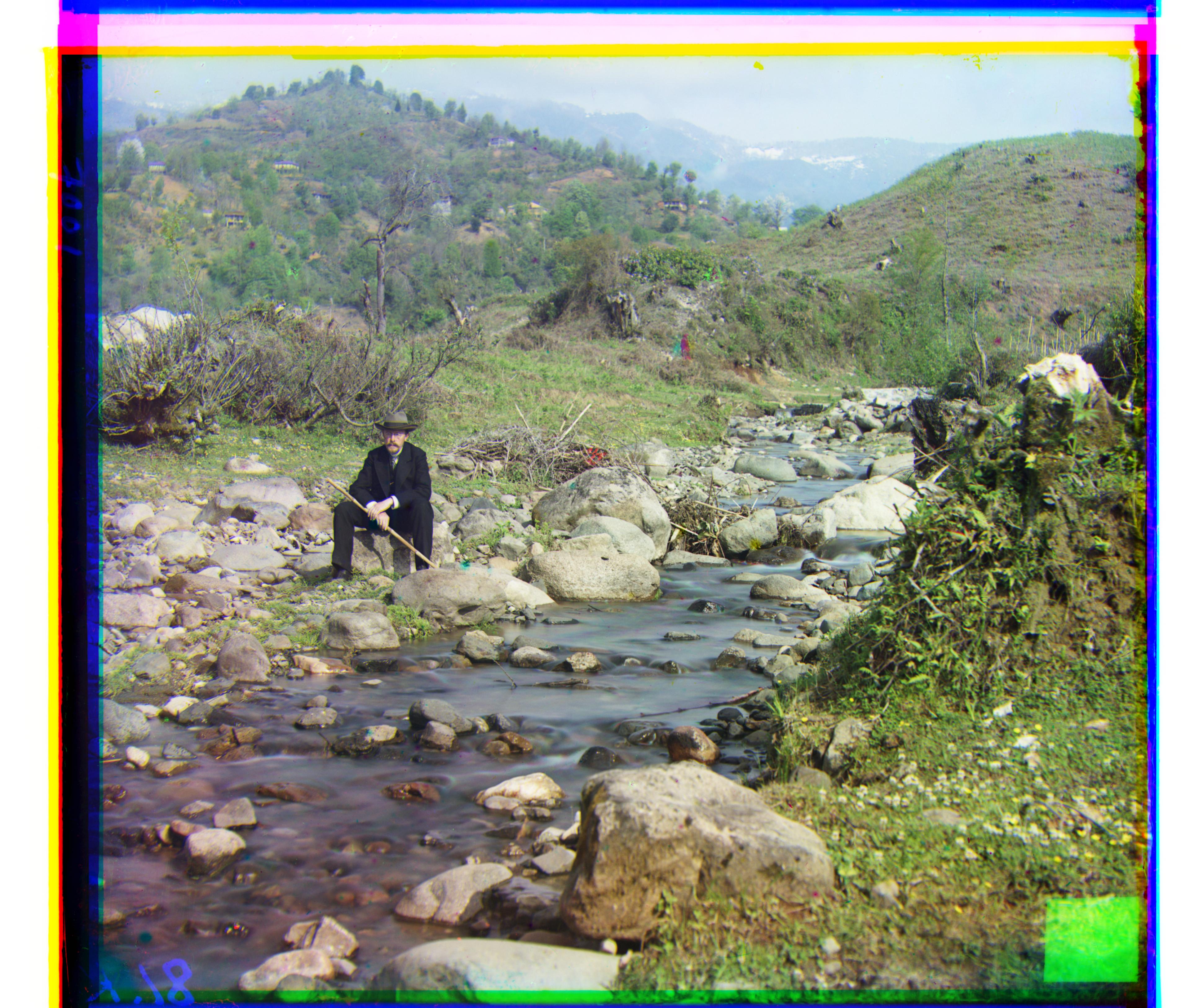
Green: (79, 29)
Red: (176, 37)
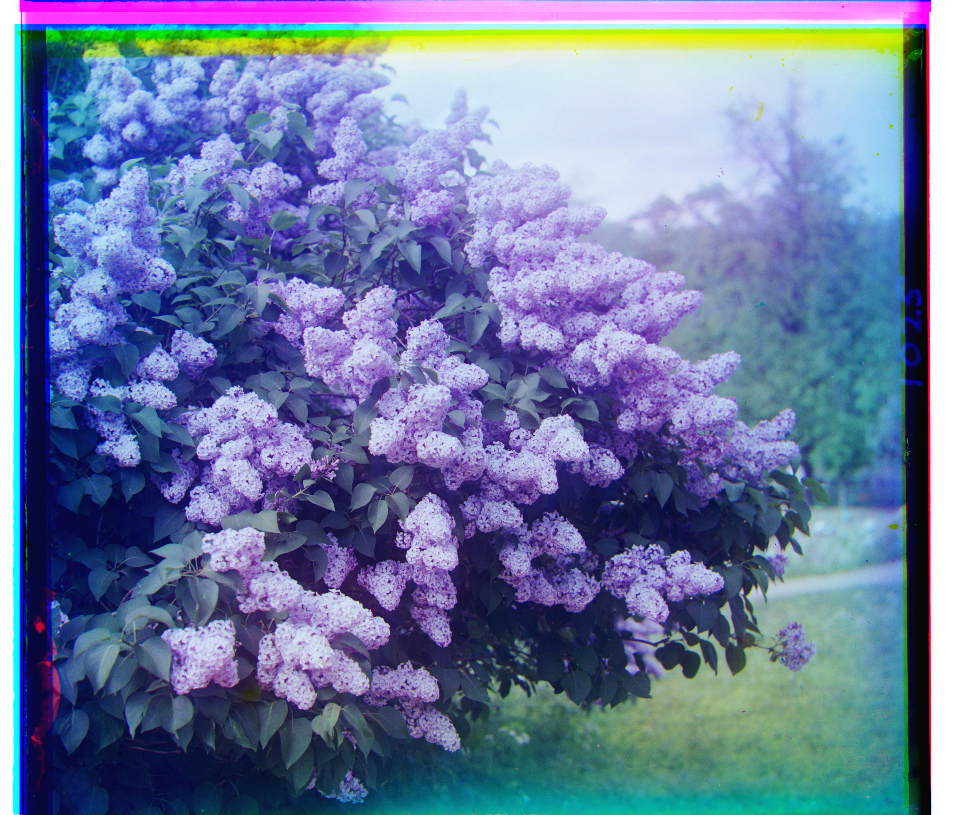
Green: (49, -6)
Red: (96, -25)
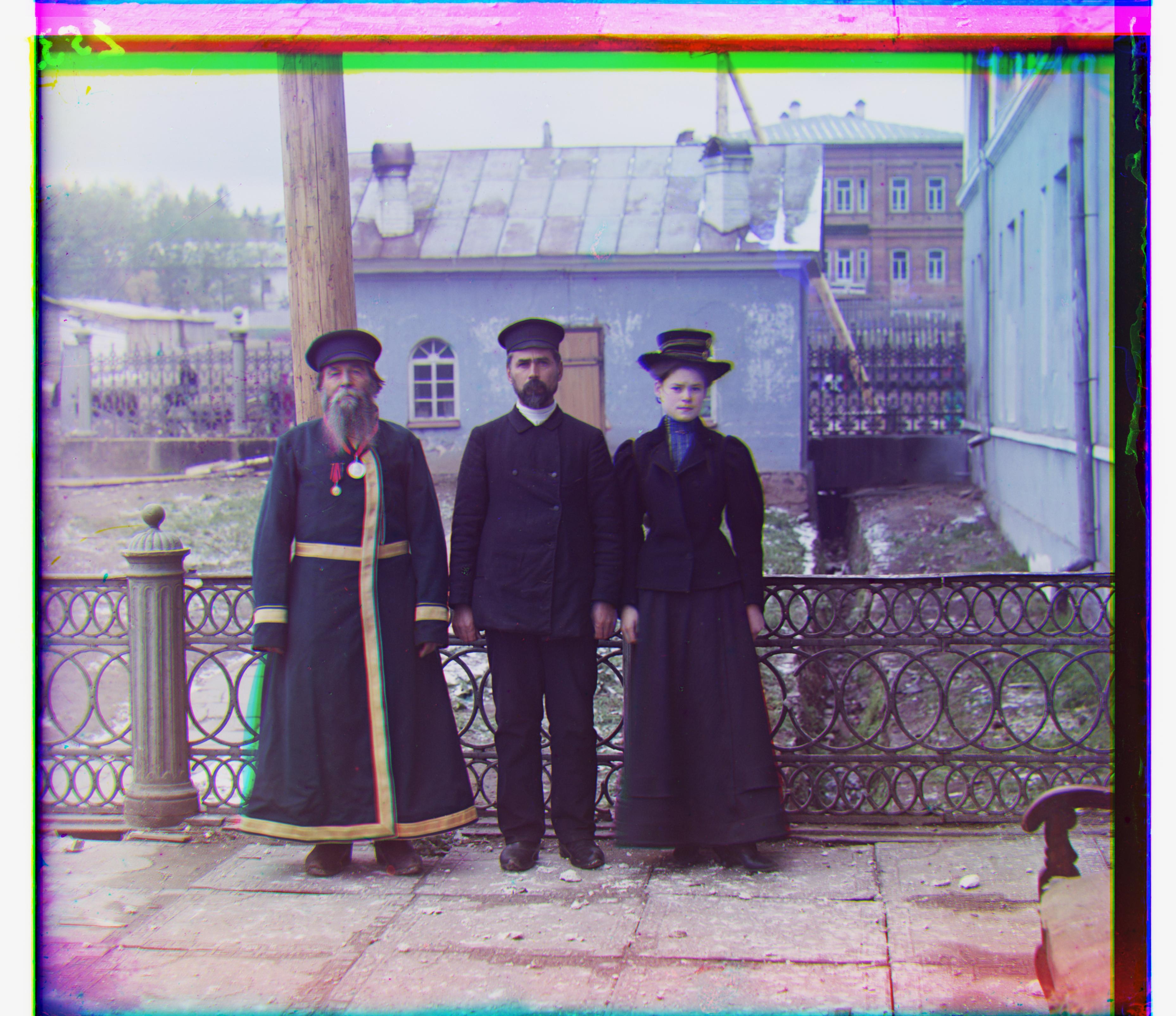
Green: (53, 14)
Red: (112, 11)
Green: (3, 3)
Red: (6, 3)
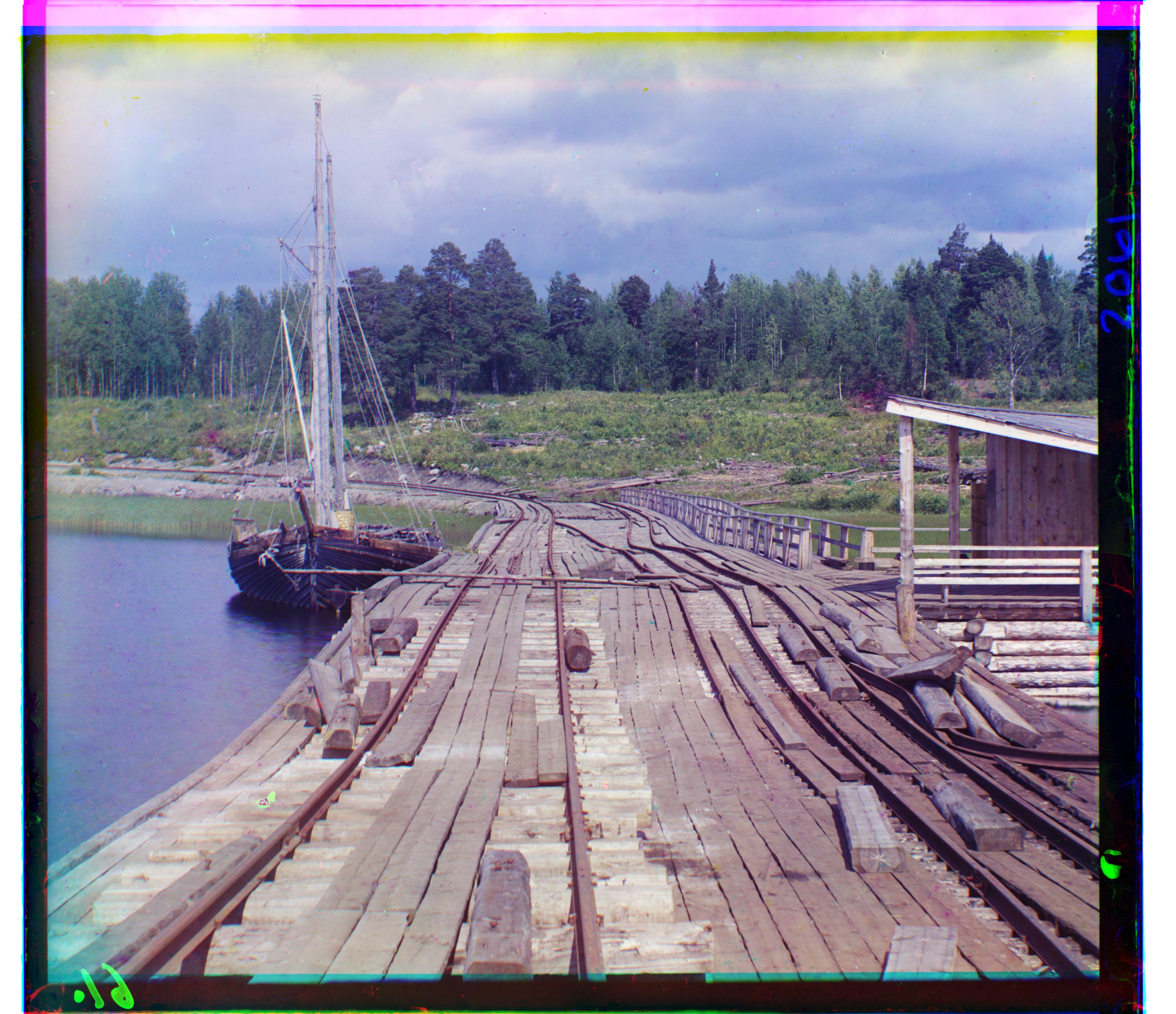
Green: (15, -7)
Red: (83, -16)
Pyramid Results for Additional Images
I also ran the same algorithm on three additional images.
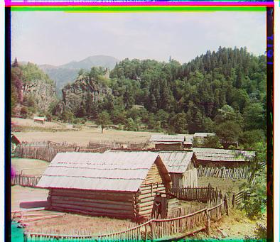
Green: (3, 0)
Red: (10, 0)
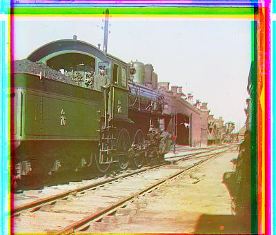
Green: (4, 3)
Red: (30, -17)
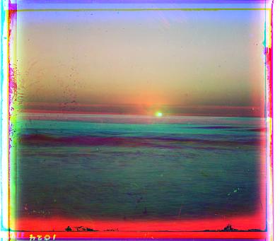
Green: (5, 1)
Red: (-4, -10)
Alignment Failure
Emir’s red channel is misaligned. The algorithm selects a green shift of (49, 24) and a red shift of (378, −481). Applying the red shift leaves a separate red outline of the figure far from the other channels.
A likely cause is the difference in the coat’s brightness across exposures. The blue coat appears bright through the blue filter and dark through the red filter. Mean subtraction and normalization help with overall brightness differences, but this local difference can lead raw-pixel NCC to favor an incorrect shift. Once the pyramid selects a poor estimate at a smaller level, the ±2 refinement window at each larger level may be too narrow to recover the correct alignment.