Project 2: Fun with filters and frequencies!
Part 1: Fun with Filters
Part 1.1: Convolutions from Scratch!
For each output pixel, convolution multiplies a neighborhood of image pixels by a flipped filter and adds the products. I wrote two NumPy implementations. The first uses four loops: two over the image and two over the filter. The second keeps the image loops and uses NumPy to multiply and sum each neighborhood.
Both functions flip the filter horizontally and vertically. I add zero padding before convolution so the output has the same dimensions as the input. For an even filter dimension, the padding has one more pixel before the image than after it. This matches SciPy’s mode="same" alignment. Zero padding treats pixels outside the image as black, so the box blur darkens the border.
Four loops
def convolve_four_loops(image, kernel):
    # Get image and filter dimensions
    height, width = image.shape
    kh, kw = kernel.shape

    # Flip filter vertically and horizontally
    flipped = kernel[::-1, ::-1]

    # Add zero padding so output keeps original image size
    padded = np.pad(image, ((kh // 2, (kh - 1) // 2), (kw // 2, (kw - 1) // 2)), mode="constant")

    # Create empty output image
    output = np.zeros((height, width))

    # Visit each output pixel
    for row in range(height):
        for col in range(width):
            # Multiply each nearby pixel by its filter weight
            for i in range(kh):
                for j in range(kw):
                    output[row, col] += padded[row + i, col + j] * flipped[i, j]

    return output
Two loops
def convolve_two_loops(image, kernel):
    # Get image and filter dimensions
    height, width = image.shape
    kh, kw = kernel.shape

    # Flip filter vertically and horizontally
    flipped = kernel[::-1, ::-1]

    # Add zero padding so output keeps original image size
    padded = np.pad(image, ((kh // 2, (kh - 1) // 2), (kw // 2, (kw - 1) // 2)), mode="constant")

    # Create empty output image
    output = np.zeros((height, width))

    # Visit each output pixel
    for row in range(height):
        for col in range(width):
            # Select image neighborhood covered by filter
            patch = padded[row:row + kh, col:col + kw]
            # Multiply corresponding values + add products
            output[row, col] = np.sum(patch * flipped)

    return output
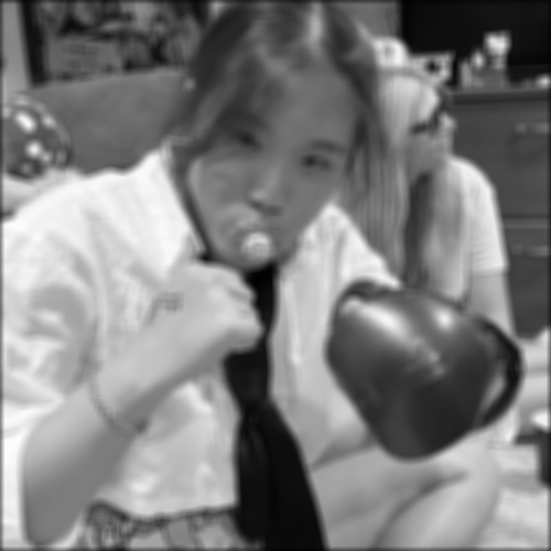
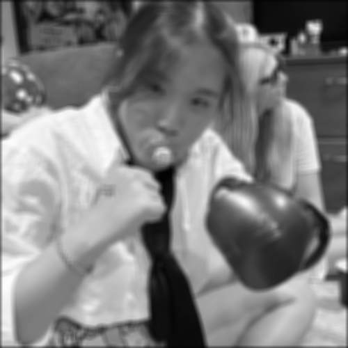
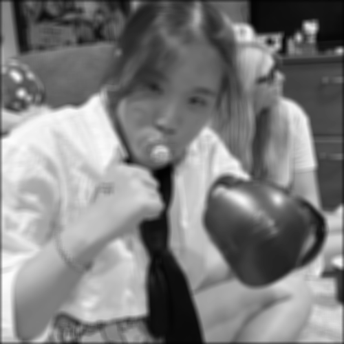
My 9 × 9 box filter gives all 81 pixels equal weight. Dividing by 81 keeps its weights summed to 1. I apply it to my 500 × 500 selfie and compare the outputs with scipy.signal.convolve2d using the same padding.
# Define 9x9 box filter
box_filter = np.ones((9, 9)) / 81
# Apply box filter with four loops + measure runtime
start = perf_counter()
blurred_four = convolve_four_loops(selfie, box_filter)
four_time = perf_counter() - start
print(f"Four-loop runtime: {four_time:.3f} seconds")
# Display blurred image
plt.imshow(blurred_four, cmap="gray", vmin=0, vmax=1)
plt.title("9x9 box blur: four loops")# Apply box filter with two loops + measure runtime
start = perf_counter()
blurred_two = convolve_two_loops(selfie, box_filter)
two_time = perf_counter() - start
print(f"Two-loop runtime: {two_time:.3f} seconds")
# Display blurred image
plt.imshow(blurred_two, cmap="gray", vmin=0, vmax=1)
plt.title("9x9 box blur: two loops")# Apply box filter with SciPy + measure runtime
start = perf_counter()
blurred_scipy = convolve2d(selfie, box_filter, mode="same", boundary="fill", fillvalue=0)
scipy_time = perf_counter() - start
print(f"SciPy runtime: {scipy_time:.3f} seconds")
# Compare pixel values with SciPy
print("Four loops match SciPy:", np.allclose(blurred_four, blurred_scipy))
print("Two loops match SciPy:", np.allclose(blurred_two, blurred_scipy))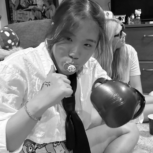
| Implementation | Time (seconds) |
|---|---|
| Four loops | 5.341 |
| Two loops | 0.570 |
| SciPy | 0.023 |
I use np.allclose to compare pixel values. Both implementations match SciPy within its default tolerance. The two-loop version is faster because NumPy handles the inner multiplication and sum. SciPy is fastest in this run.
I also convolve the selfie with finite difference filters. Dx measures changes across columns, so vertical boundaries appear strongly. Dy measures changes across rows, so horizontal boundaries appear strongly. In the derivative displays, gray is zero, white is positive, and black is negative.
# Define finite-difference filters
dx = np.array([[1, -1]])
dy = np.array([[1], [-1]])
# Apply finite-difference filters with two loops
selfie_dx = convolve_two_loops(selfie, dx)
selfie_dy = convolve_two_loops(selfie, dy)
# Display horizontal brightness changes
plt.figure()
plt.imshow(selfie_dx, cmap="gray", vmin=-1, vmax=1)
plt.title("Selfie: Dx")
# Display vertical brightness changes
plt.figure()
plt.imshow(selfie_dy, cmap="gray", vmin=-1, vmax=1)
plt.title("Selfie: Dy")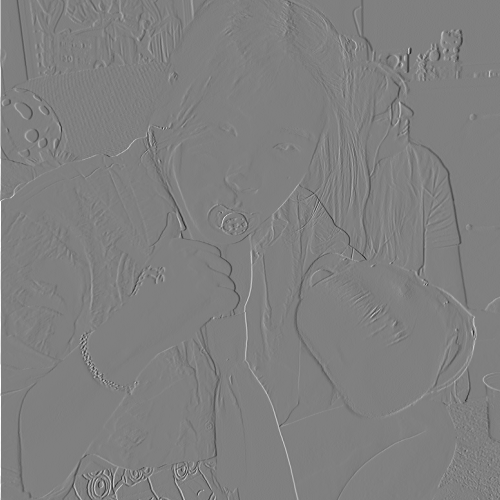
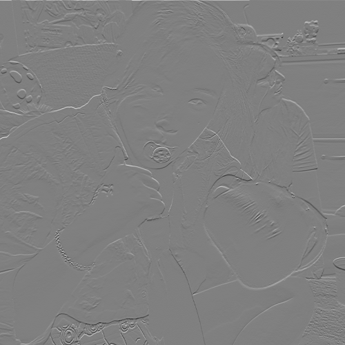
Part 1.2: Finite Difference Operator
I apply the same Dx and Dy filters to the cameraman image with SciPy. Here I use symmetric boundary extension, which mirrors values at the image border. I combine the derivatives with the gradient magnitude, √(Ix² + Iy²), to measure edge strength in either direction.
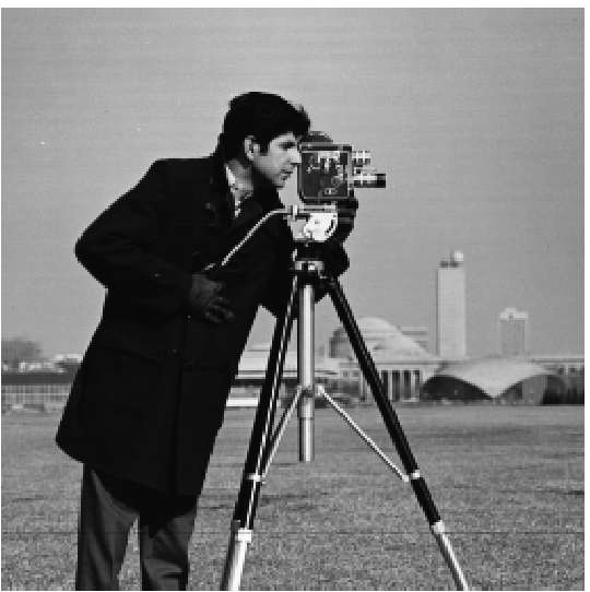
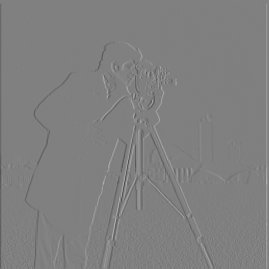
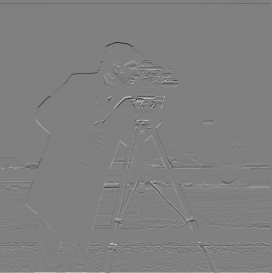
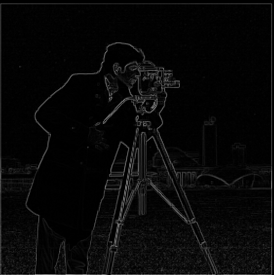
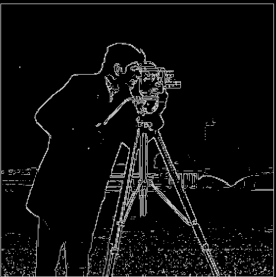
I binarize the magnitude with gradient_magnitude > 0.15. This keeps the camera and much of the person’s outline while removing many small responses in the grass. Some grass remains, and some weak edges disappear. I chose this threshold to reduce the background detail without losing too much of the subject.
Part 1.3: Derivative of Gaussian (DoG) Filter
Finite differences respond to small changes in brightness, including texture in the grass. I first smooth the image with a Gaussian filter. I use cv2.getGaussianKernel(19, 3) and multiply the column by its transpose to make a 19 × 19 filter with σ = 3. Pixels near the center receive more weight than pixels near the edge.

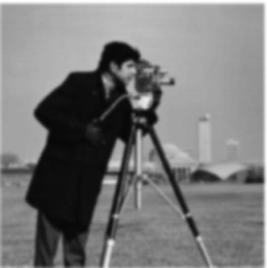
I take finite differences of the smoothed image and calculate the gradient magnitude again. Smoothing reduces fine texture and spreads the remaining edges over more pixels. It also lowers their peak strength, so I use a smaller threshold of 0.03. A threshold of 0.04 removed more of the outline than I wanted.
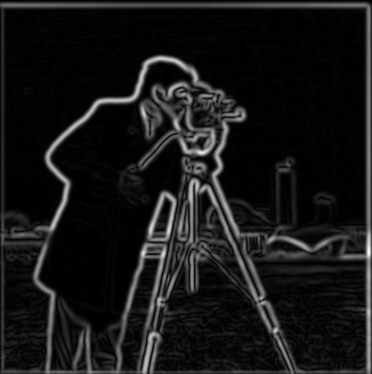
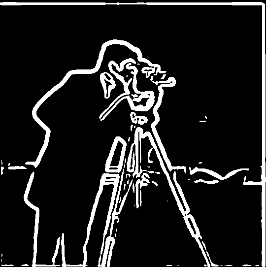
I then convolve the Gaussian filter with Dx and Dy using mode="full". These derivative of Gaussian (DoG) filters combine smoothing and differentiation. Convolution is associative: (I ∗ G) ∗ D = I ∗ (G ∗ D). I can apply each DoG filter directly to the original cameraman image.


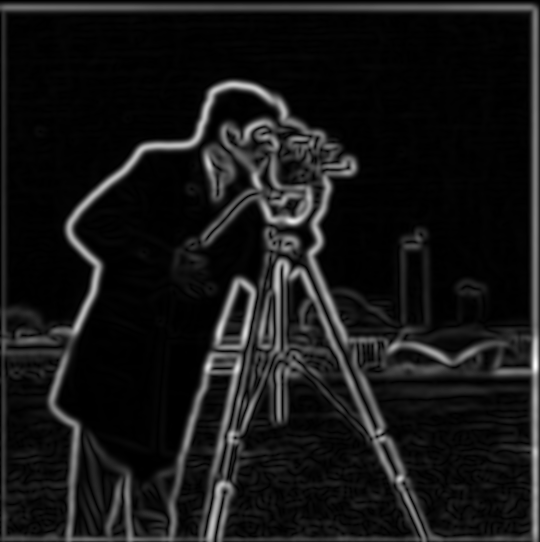
The x derivatives, y derivatives, and gradient magnitudes from the two methods all pass np.allclose in my notebook. Compared with Part 1.2, both methods reduce the grass texture and produce wider, smoother edges. The magnitude images use their own display ranges so the edge structure is visible.
Part 2: Fun with Frequencies!
Part 2.1: Image "Sharpening"
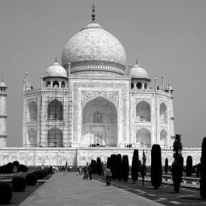
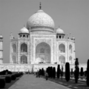
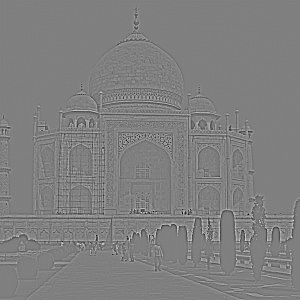
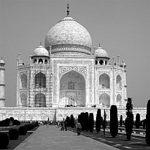
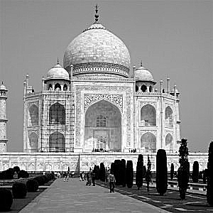
A Gaussian blur reduces fine detail. I subtract the blurred image from the original to isolate high frequencies, then add a scaled copy of those details back to the original. The sharpened image is I + α(I − G ∗ I). Here, I is the original image, G is the Gaussian blur filter, and ∗ means convolution. G ∗ I is the blurred image, so I − G ∗ I contains the high-frequency details. The sharpening amount α controls how much of that detail I add back. With α = 0, the image stays unchanged; larger positive values increase the sharpening.
I combine these operations into one convolution with the filter (1 + α)δ − αG. The impulse filter δ has a 1 at its center and zeros elsewhere, so convolving it with I returns I unchanged. This combined filter produces (1 + α)I − α(G ∗ I), which is the same sharpening formula written above.
I use a 7 × 7 Gaussian with σ = 1 and symmetric boundary extension. After sharpening, I clip values to [0, 1]. The high-frequency displays use gray for zero so both positive and negative details remain visible.
Taj Mahal
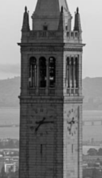
Berkeley
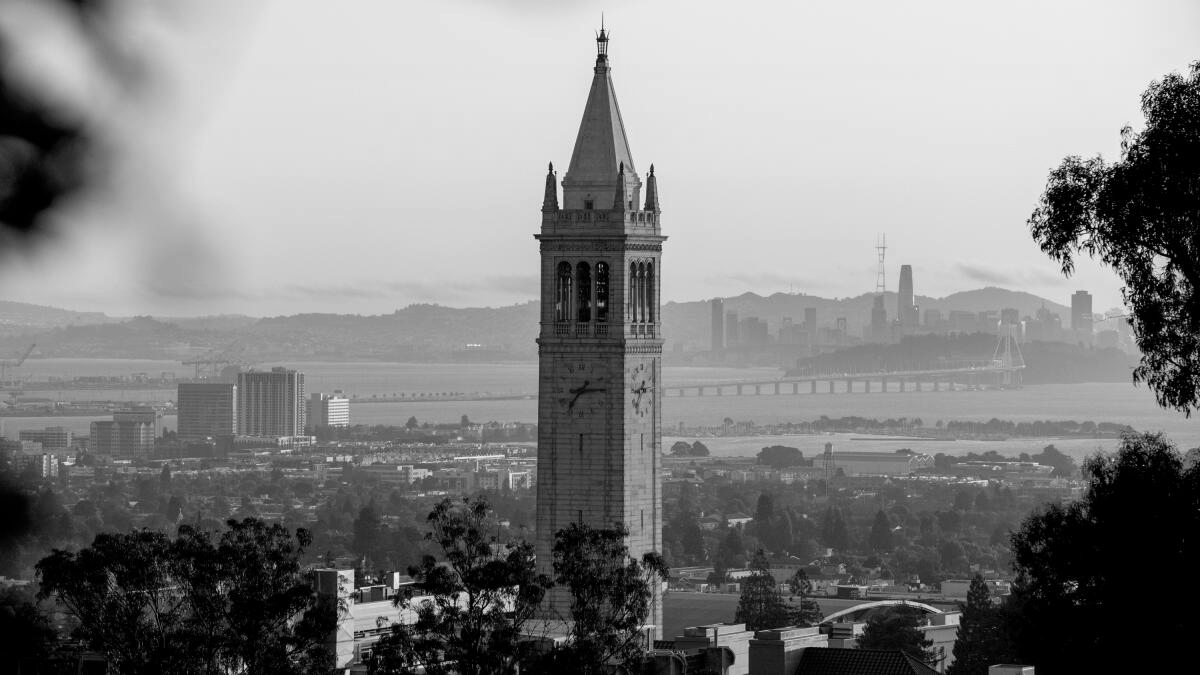
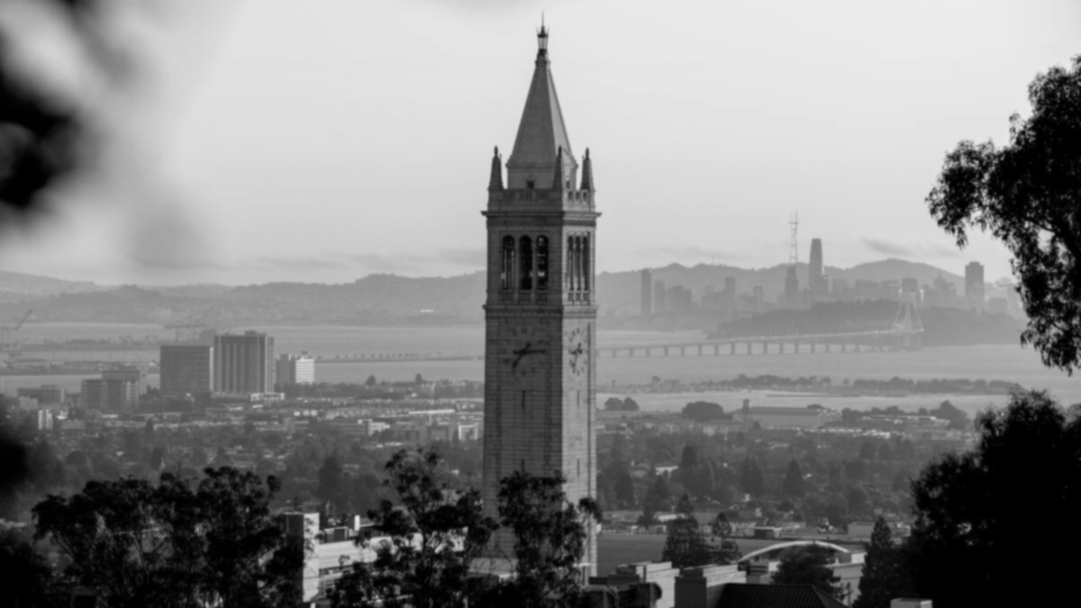
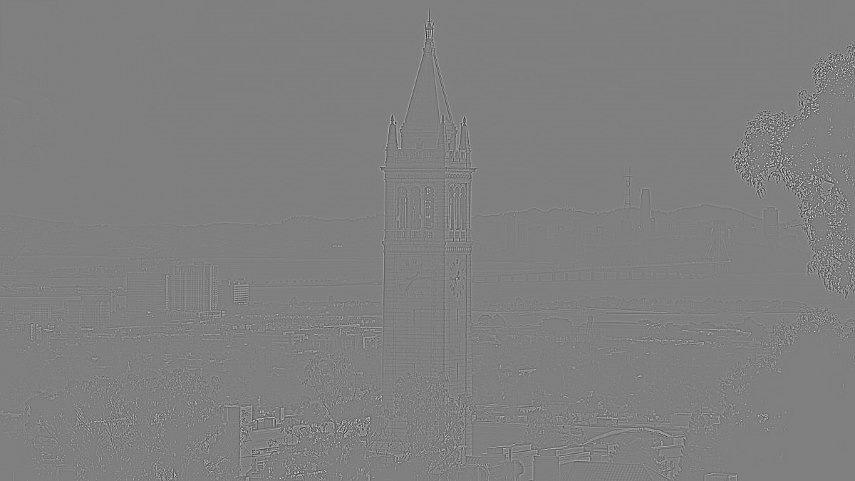
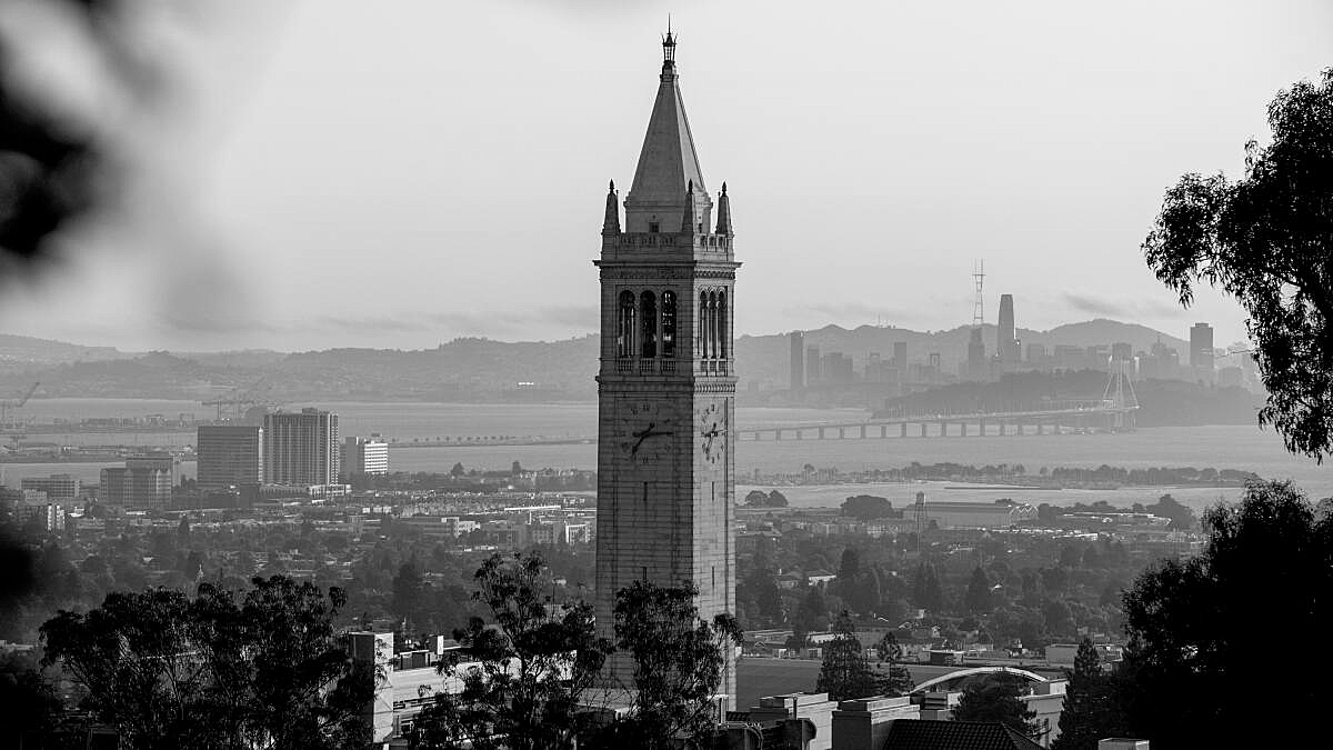
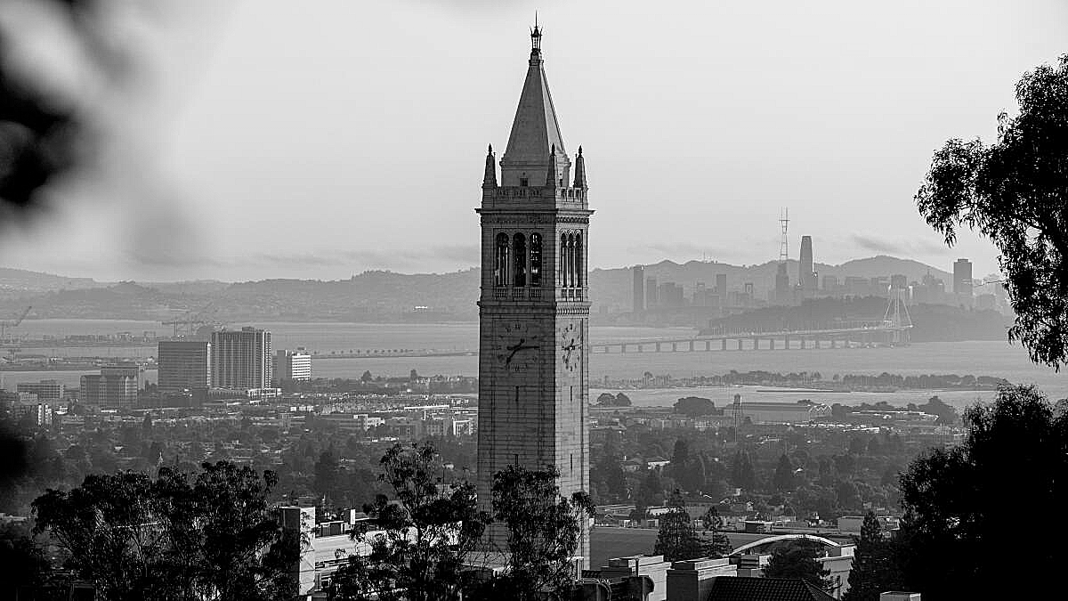
Increasing α strengthens contrast around edges. At α = 2, the building details stand out more, but bright and dark outlines also become stronger. Sharpening can exaggerate existing texture.
Blur, then sharpen
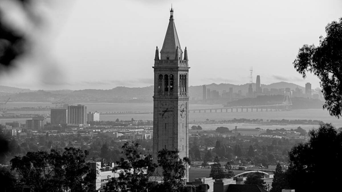
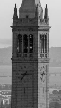
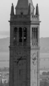
I blur the Berkeley image with the same Gaussian, then sharpen that blurred image with α = 2. The result has stronger boundaries than the blurred image. Fine detail lost during blurring is still missing. The full images make the overall change look small, so I also compare the same crop from each image.
Part 2.2: Hybrid Images
A hybrid image combines the low frequencies of one image with the high frequencies of another. I blur the first image to keep its low frequencies. I subtract a blurred copy of the second image from itself to keep its high frequencies, then add these two components. The first image’s broad shapes are easier to see from farther away, while the second image’s fine details are easier to see up close. This implements the Gaussian filtering method in Section 2 of Oliva, Torralba, and Schyns’s Hybrid Images.
I use the starter align_images function and select corresponding eyes to align the faces. The function adjusts position, scale, and rotation, then crops the images to a shared size. This follows the paper’s discussion in Section 2.2: matching features and pose helps the two images form a coherent face.
Each Gaussian extends three standard deviations from its center. I filter vertically and horizontally with symmetric boundary extension. The σ values below are in pixels after alignment. A larger σ makes a wider blur and a lower low-pass cutoff. For the high-pass component, subtracting that wider blur retains a broader range of detail.
Derek and Nutmeg
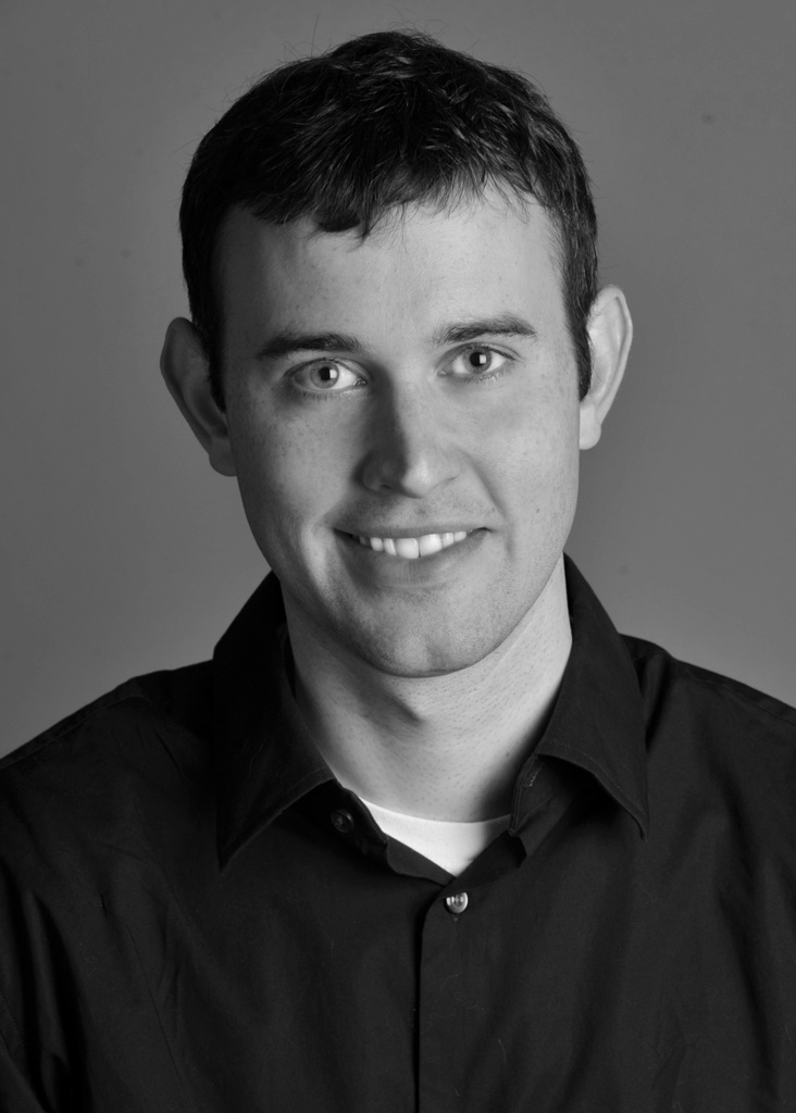
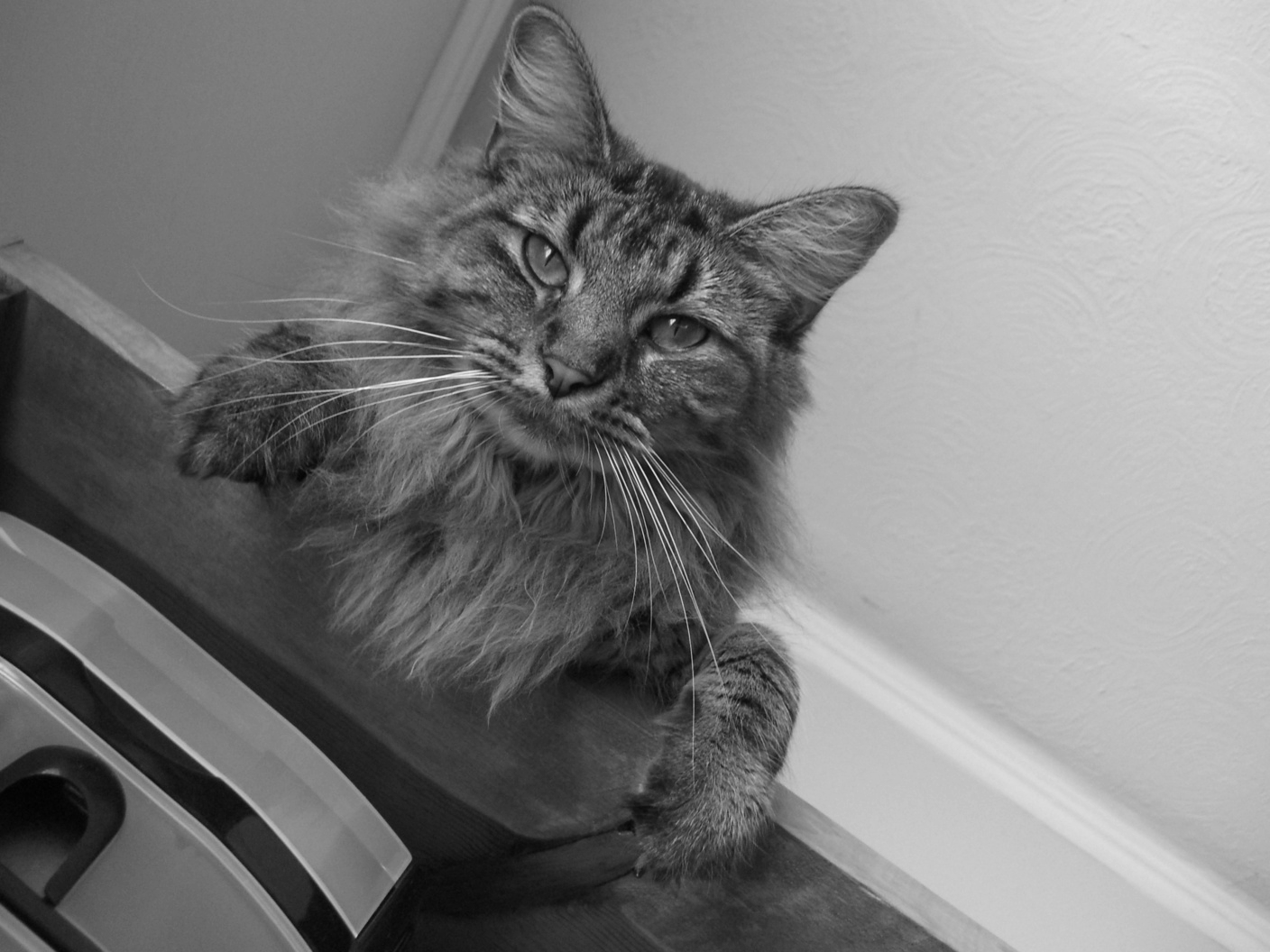
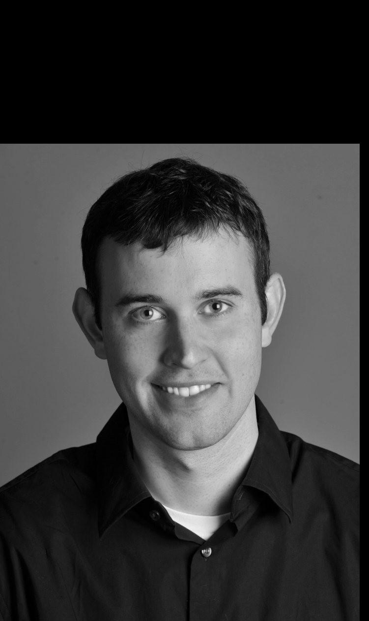
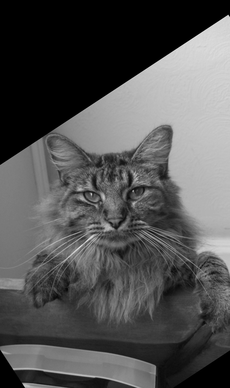
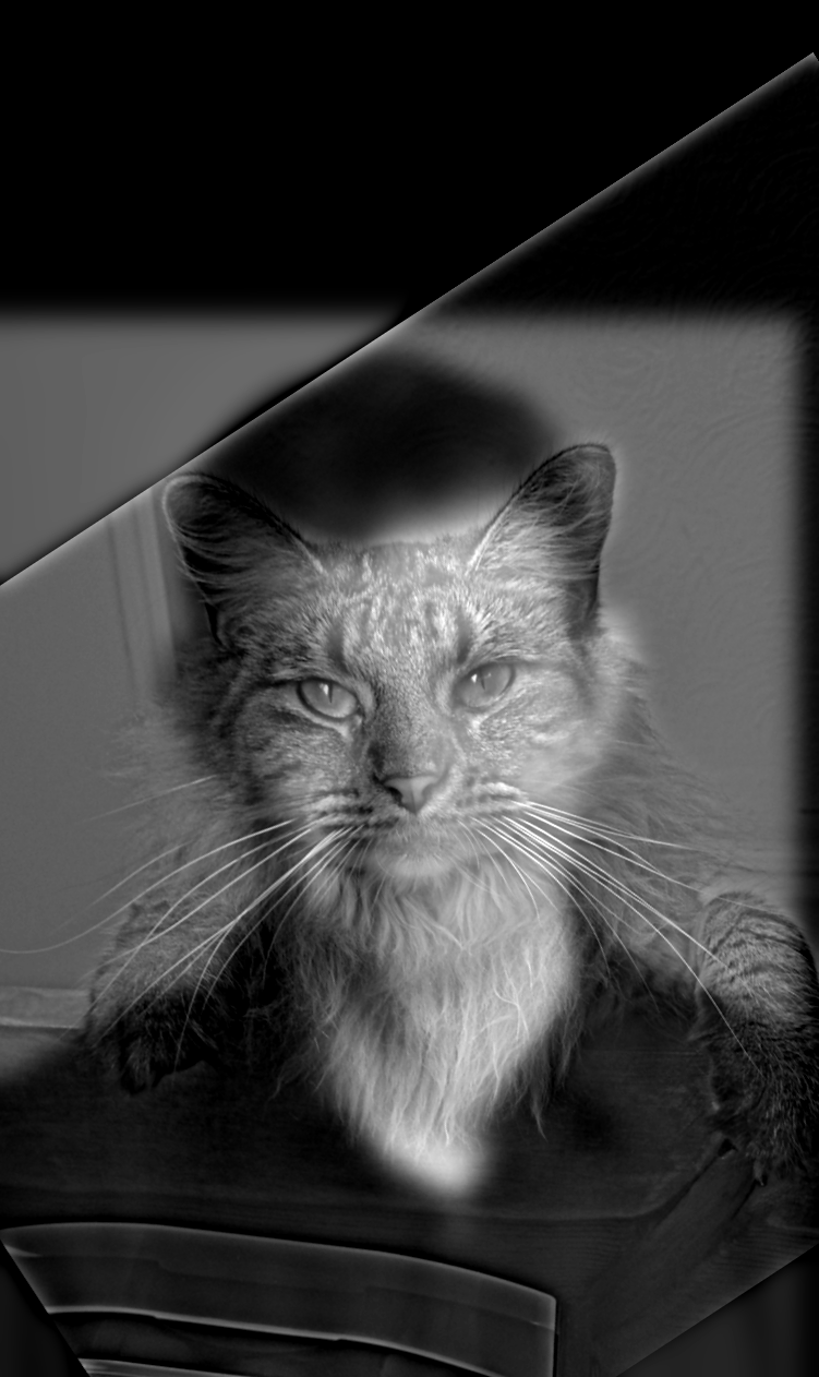
Derek supplies low frequencies with σ = 12, and Nutmeg supplies high frequencies with σ = 8. I pass Nutmeg first to the alignment function so the rotation adjusts Nutmeg toward Derek’s pose. Nutmeg’s eyes and fur are visible up close; Derek’s face becomes clearer when I step back.
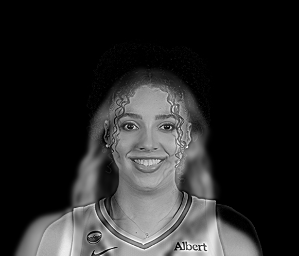
Paige and Azzi
Paige and Azzi are my favorite pair. Paige supplies the low frequencies with σ = 4, and Azzi supplies the high frequencies with σ = 3. I first tried σ = 6 for Paige, but her face was too faint. Reducing it to 4 kept more of her facial structure.
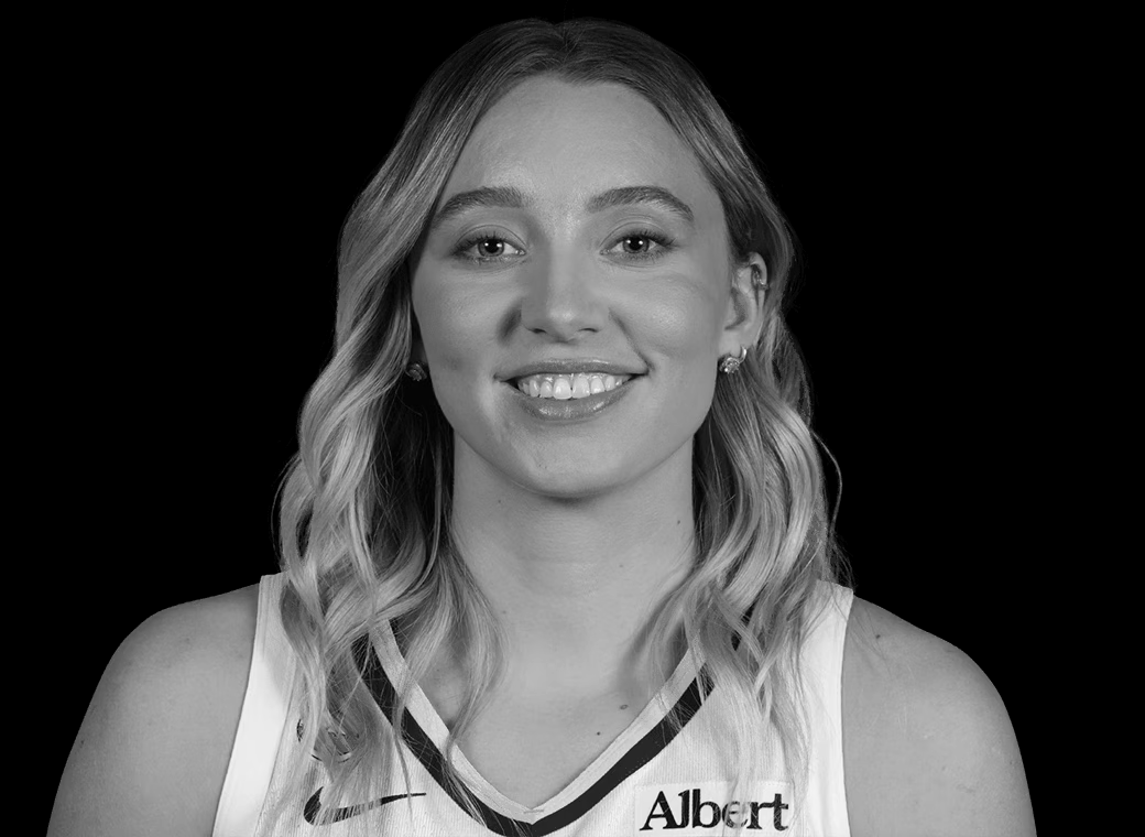
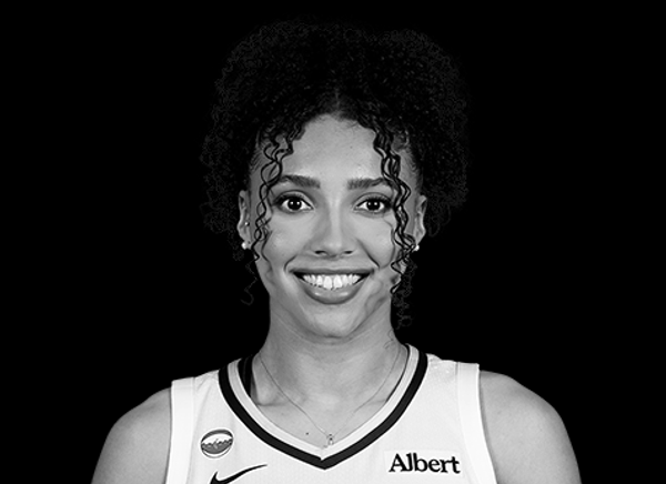
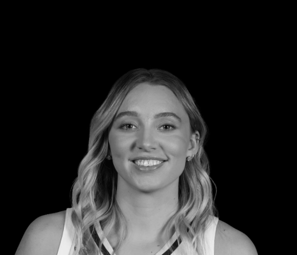
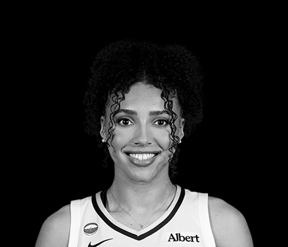
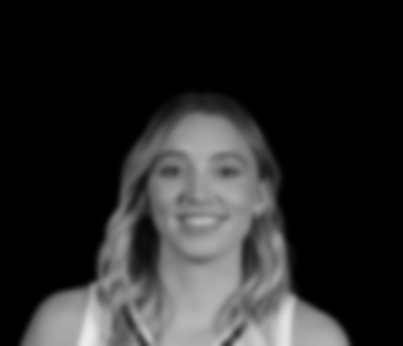
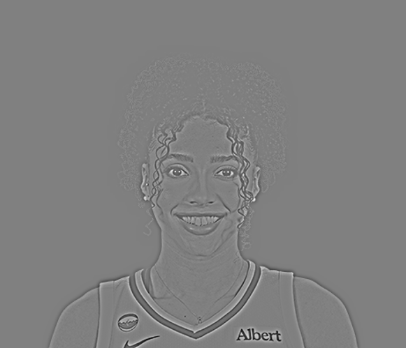
I calculate each Fourier display with log(abs(fftshift(fft2(image)))). The shift puts low frequencies at the center, and the logarithm makes weaker frequencies visible. The input transforms below use the aligned images. I display each transform with its own grayscale range.
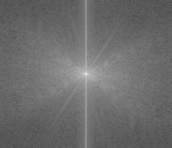
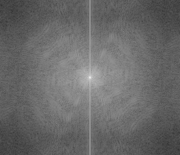
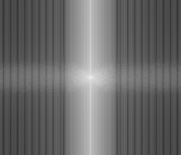
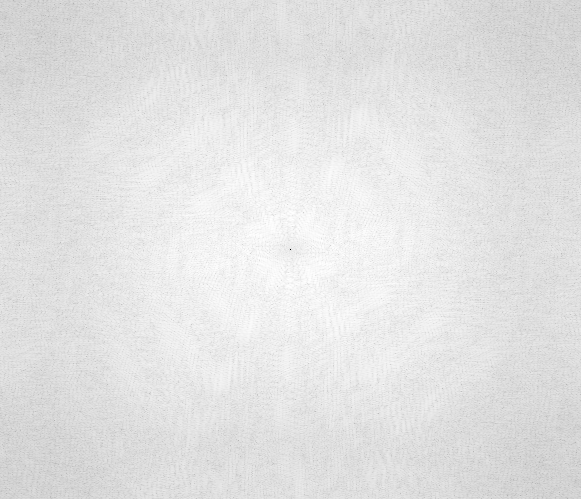
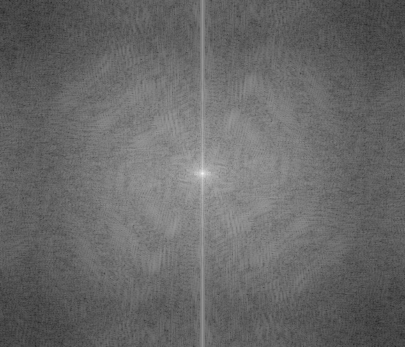
The low-pass result concentrates energy near the center. Subtracting Azzi’s blur removes low frequencies, while her edges remain in the high-pass result. The final hybrid contains both components. Their mouths and face outlines do not align perfectly, so some doubled features remain visible up close.
Josh and Rushil
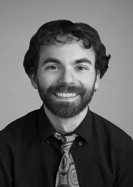
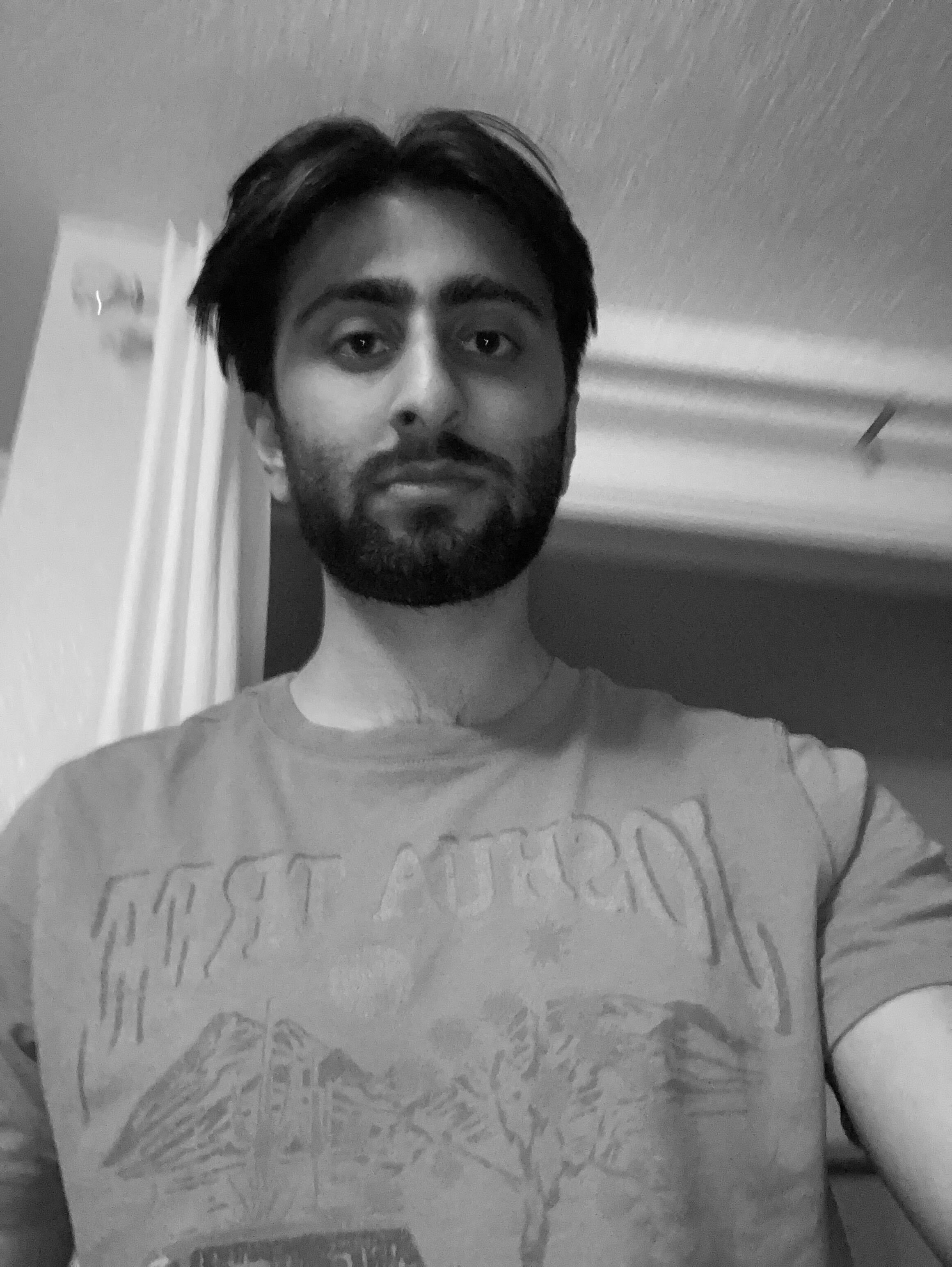
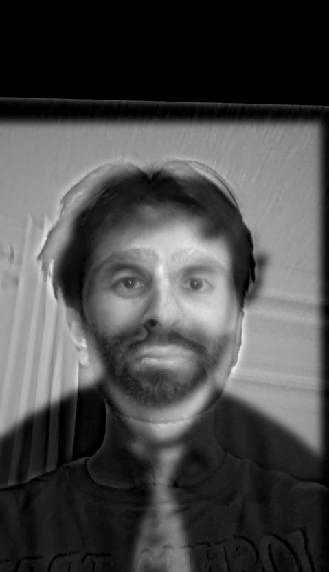
Josh supplies low frequencies with σ = 6, and Rushil supplies high frequencies with σ = 6. Rushil was hard to see with a high-pass σ of 3. Increasing it to 6 retained more of his face, while Josh remained visible from farther away. These settings differ from Paige and Azzi because the aligned faces have different scales and details.
Part 2.3: Gaussian and Laplacian Stacks
I build six Gaussian levels for each fruit. Level 0 is the original image. To create each next level, I blur the previous one with σ = 2, 4, 8, 16, and 32 in order. These are successive blur widths, so each level includes the smoothing from earlier levels. Every level keeps the original 300 × 300 dimensions.
This uses the scale separation described in Section 2 of Burt and Adelson’s A Multiresolution Spline With Application to Image Mosaics. Their pyramids reduce image dimensions between levels. My stacks retain the full dimensions, as the project requires.
Gaussian stacks
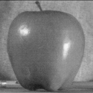
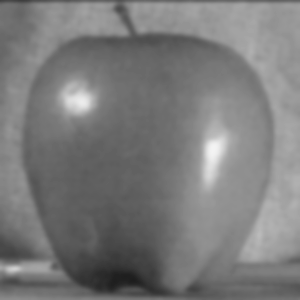
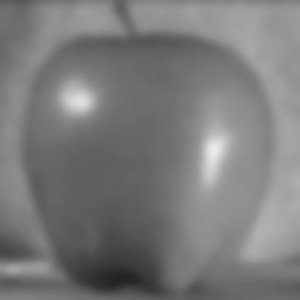
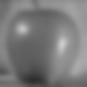

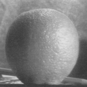
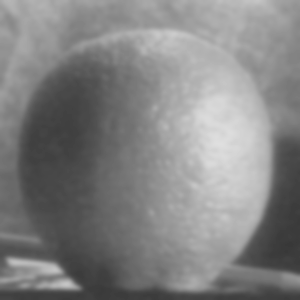
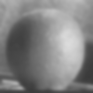
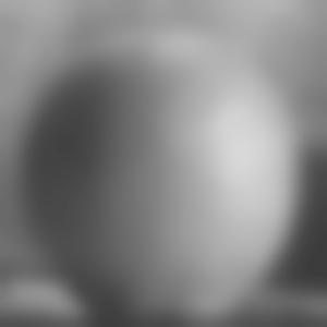

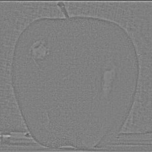
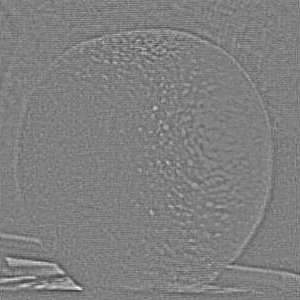
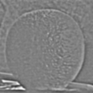
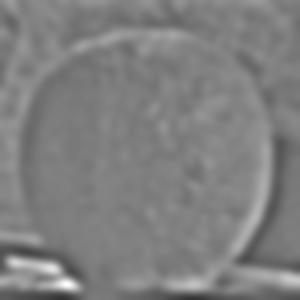
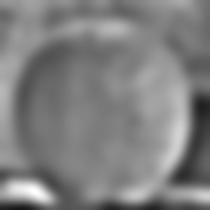
For Laplacian levels 0 through 4, I subtract each next Gaussian level from the current level: Li = Gi − Gi+1. Level 5 stores the final blurred image. Each difference contains detail removed by that step of blurring. Adding all six levels reconstructs the original because the intermediate Gaussian terms cancel. This follows the difference and reconstruction method in Sections 2.2 and 2.3 of Burt and Adelson.
Laplacian stacks


Recreating Figure 3.42
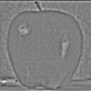
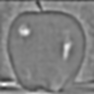
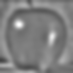
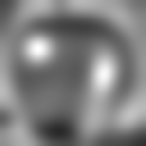
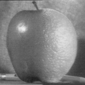
I use a mask that selects the apple on the left and the orange on the right, then build a Gaussian stack of that mask. At each level I multiply the apple’s Laplacian level by the mask and the orange’s by one minus the mask. I add the two contributions. Part 2.4 explains this blending step in more detail.
The layout below recreates panels (a) through (l) of Figure 3.42 in Szeliski’s Computer Vision: Algorithms and Applications. The first three rows contain masked Laplacian contributions at levels 0, 2, and 4. The last row sums all six levels, including levels omitted from the display.
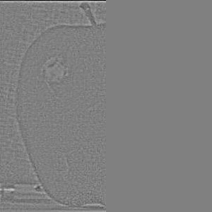
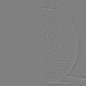
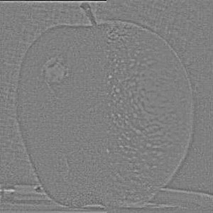
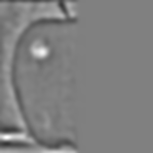
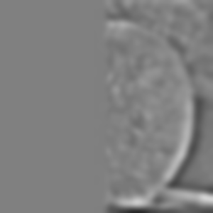
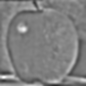
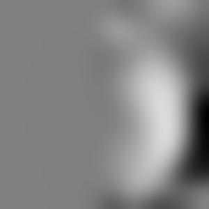
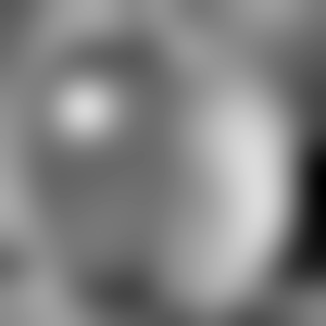
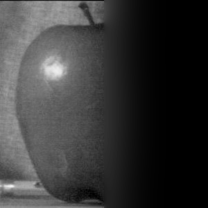
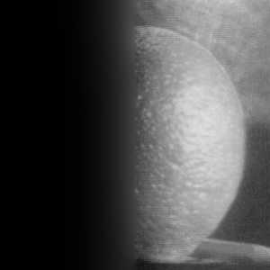
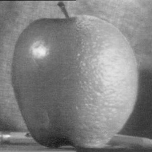
Fine edges appear in the first row. Lower rows contain broader detail, and their Gaussian masks spread the transition over more pixels. Each of the first three rows uses a shared symmetric display range across its three panels. The bottom row shows the reconstructed contributions and final blend.
Part 2.4: Multiresolution Blending (a.k.a. the Oraple!)
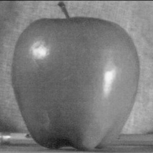
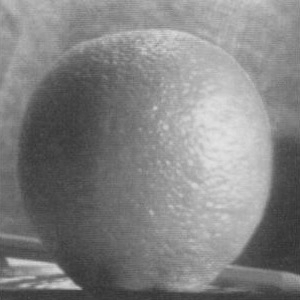
I use the mask-based blend in Section 3.2 of Burt and Adelson, on page 230. I build Gaussian stacks for the mask and both input images, then obtain Laplacian stacks for the images. At each level, Bi = MiLA,i + (1 − Mi)LB,i.
Here, i is the stack level, and A and B label the two input images. LA,i and LB,i are their Laplacian stack values at that level. Mi is the corresponding Gaussian mask level, and Bi is the blended result at that level. I multiply corresponding pixels: Mi weights image A’s contribution, and 1 − Mi weights image B’s contribution. A mask value of 1 selects A, a value of 0 selects B, and values between them mix both. The final image is the sum of Bi over all six levels.
The mask is sharper at fine levels and more blurred at coarse levels. This keeps small details near the selected boundary while mixing broad brightness changes over a wider region. Since the stacks have matching dimensions, I combine corresponding pixels directly and sum the levels.
Apple and orange







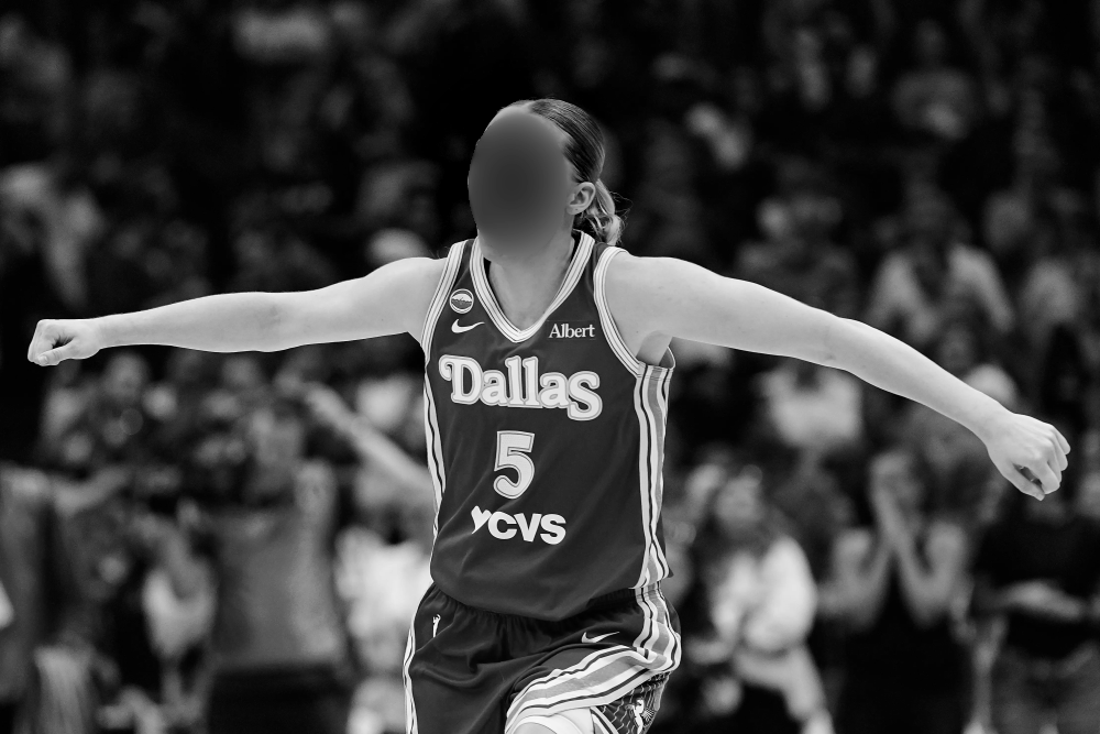
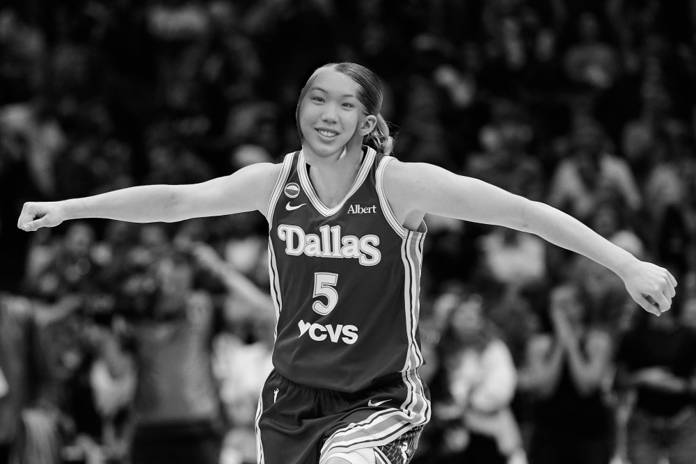
Isabel and Paige
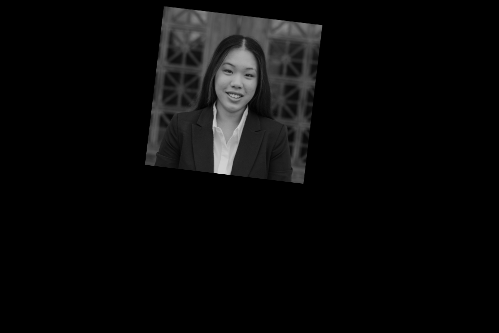
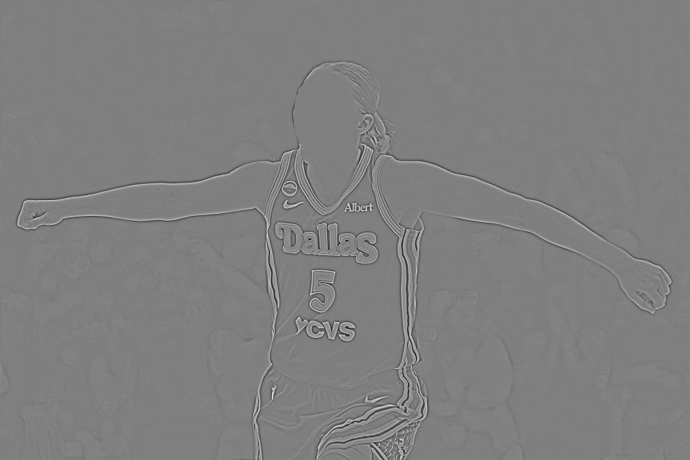
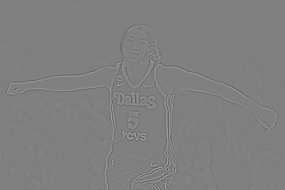
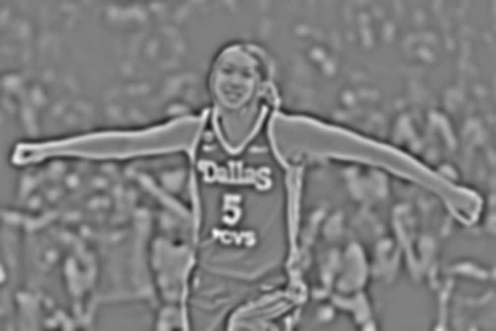
I replace Paige’s face with mine. I resize the basketball image to 1,000 pixels wide and select corresponding eyes in both images. A similarity transform scales, rotates, and moves my face into position. I then shift the target points 20 pixels right to place my face within Paige’s face area.
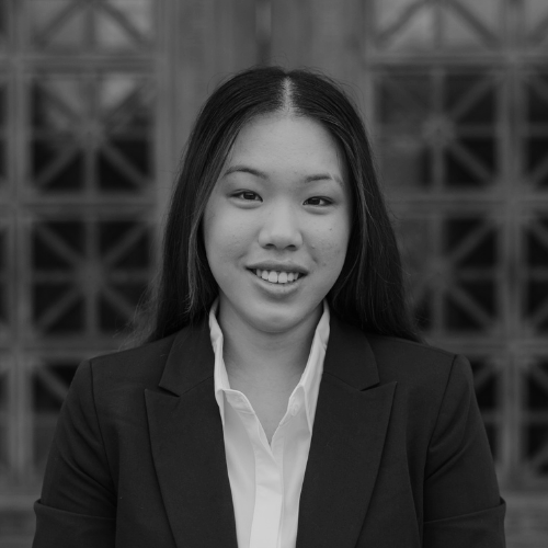
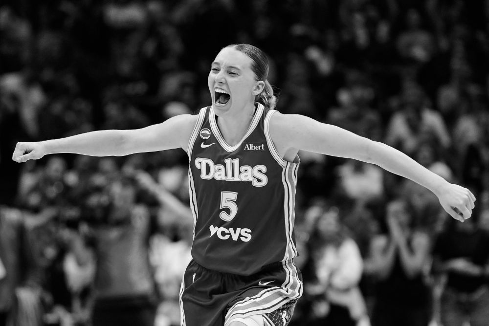
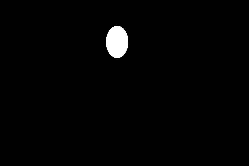
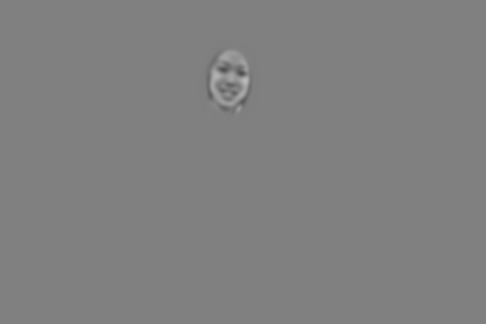
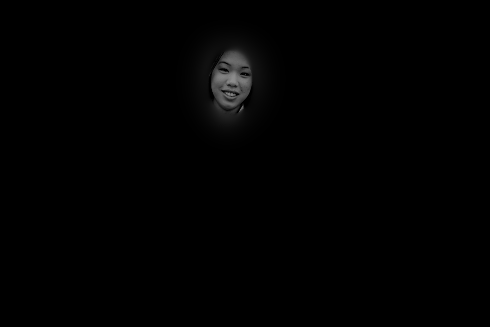
The mask is an ellipse centered at (x, y) = (470, 168), with horizontal radius 45 and vertical radius 65 pixels. White selects my face; black selects Paige’s image. The black region outside the warped selfie is padding from the transform. The mask restricts the blend to the face area.
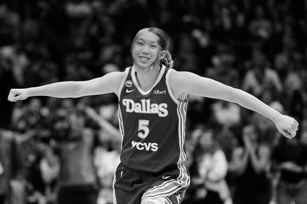
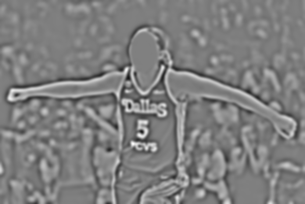
I use the same six levels and blur widths as the oraple. This keeps Paige’s pose and background while replacing the face. Some shading remains around the jaw and neck where the source faces differ.
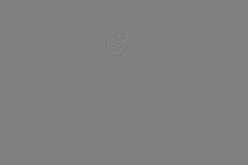
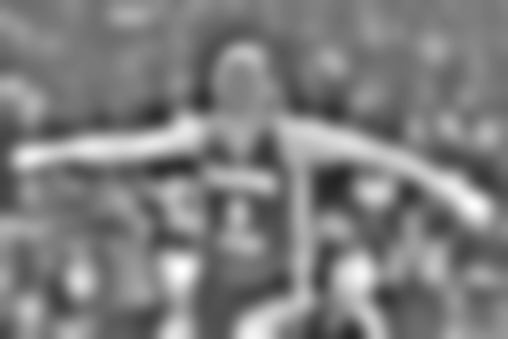
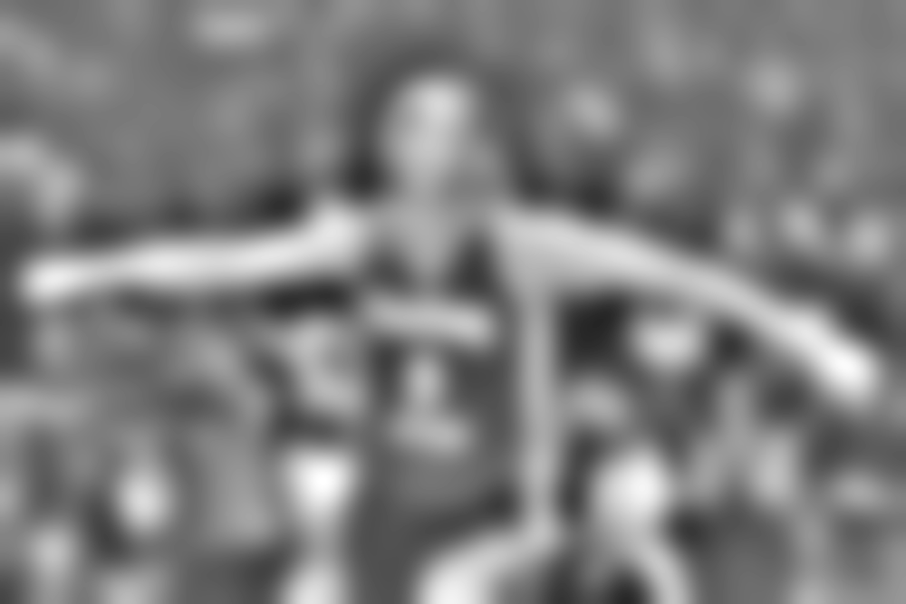
Mask and blended levels
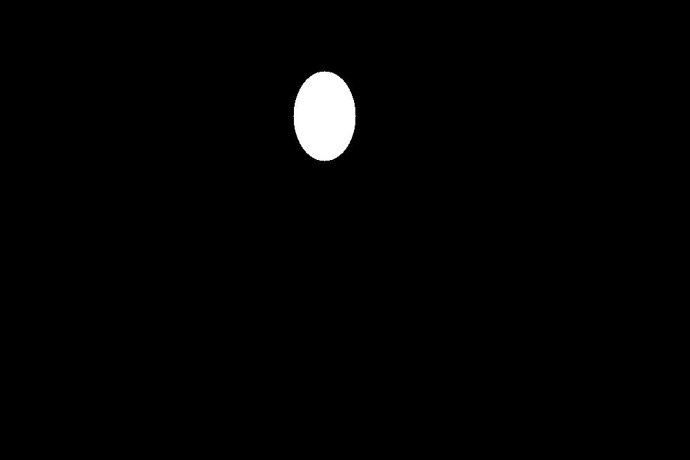
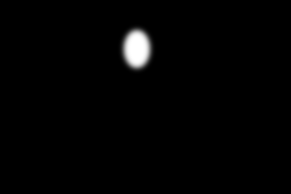
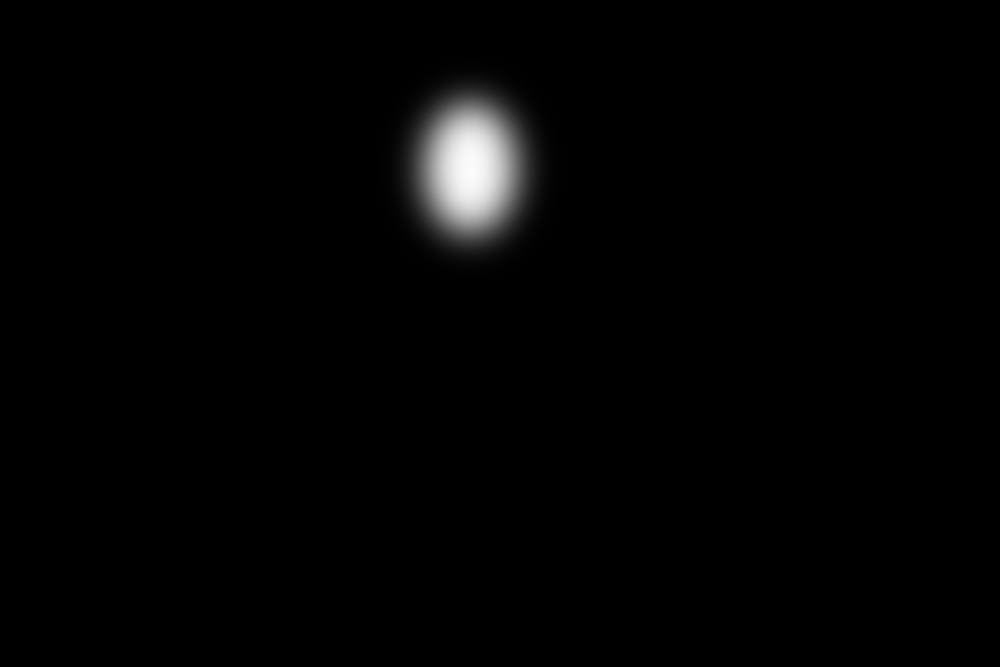
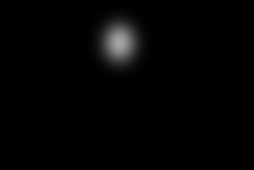
For this pair, I show the masked contributions in the same layout as Figure 10 of Burt and Adelson. Rows one through three use levels 0, 2, and 4. The last row adds all six levels. Fine facial details remain localized, while the coarser contributions mix brightness over a larger area.

Minion and Snoopy
I resize Snoopy’s image to 1,000 pixels wide and use another similarity transform to place the Minion’s face over Snoopy’s head. I select target points for the Minion’s eyes and use an ellipse centered at (500, 200), with radii 115 and 140 pixels. I blend with the same stack settings.
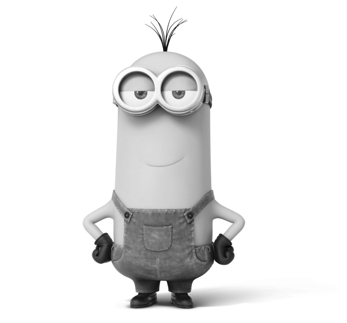
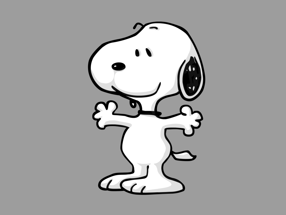
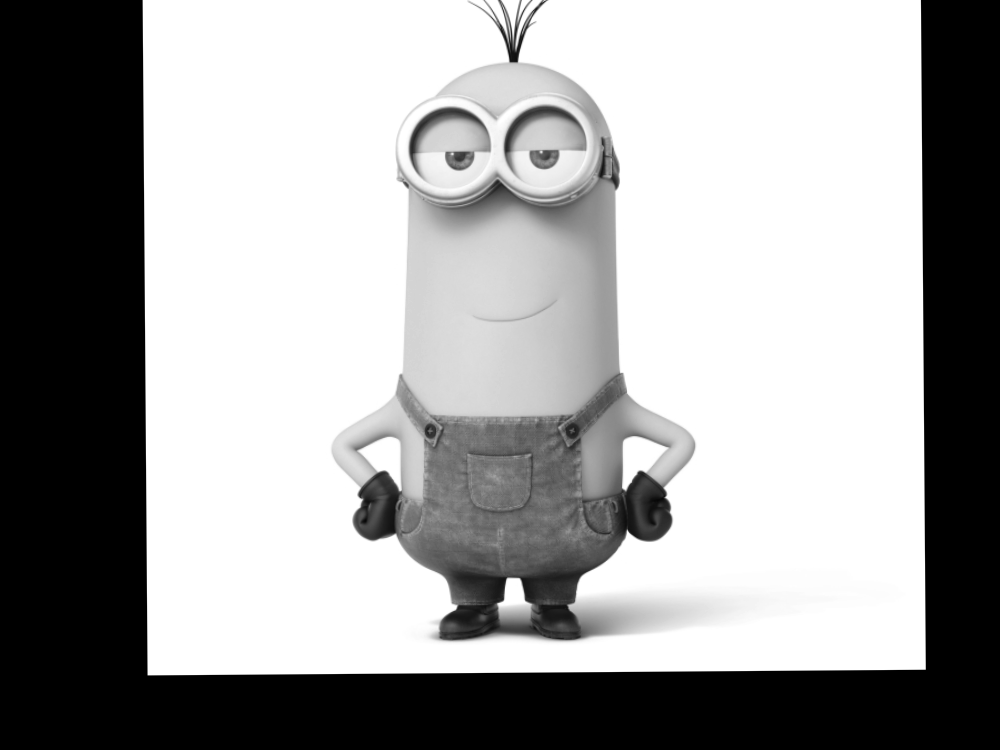
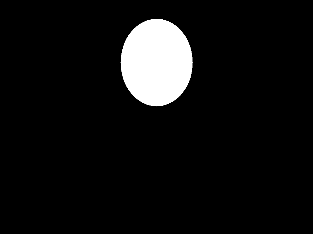
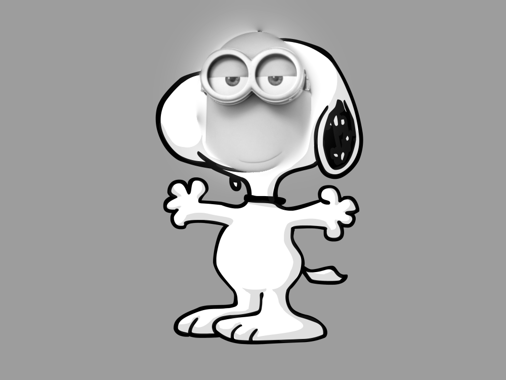
The goggles extend above Snoopy’s head, and the blend has a soft boundary around the face. Snoopy’s ears and body remain visible. Both custom blends use curved masks.
What I learned
The most important thing I learned was the difference between Gaussian and Laplacian stacks. A Gaussian level contains the image after repeated blurring. A Laplacian level contains the detail lost between two Gaussian levels. Keeping the final blurred image lets me add the Laplacian levels back together to reconstruct the original. In the blends, I can control how each level crosses the mask boundary.