Project 3: Fun with flow models
In Part A, I used a pretrained flow model to denoise, generate, and edit images. In Part B, I built UNets and trained them on MNIST, first for single-step denoising and then for flow matching.
Part A: Exploring the power of flow models
I used PixNerd with 512 × 512 inputs and RGB values in [−1, 1]. Unless stated otherwise, I used the prompt "a high quality photo" and Euler step size 0.02. For classifier-free guidance, I used w = 7 and an empty prompt for the unconditional prediction.
1. Visualizing training and sampling
1.1 Constructing noisy training inputs
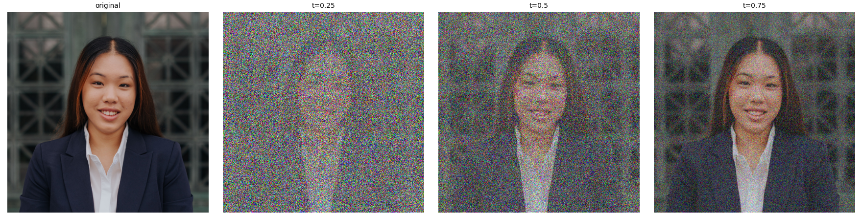
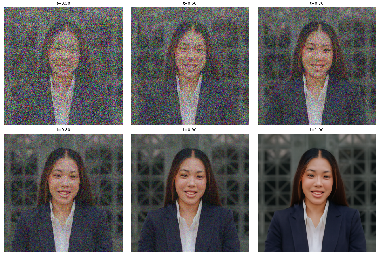
I implemented the interpolation function and used my portrait with the supplied experiment loop, which reuses one Gaussian noise tensor ε for all three times. The interpolation is xₜ = (1 − t)ε + tx₁, where x₁ is the clean image. Increasing t keeps more of the portrait. The supplied endpoint checks passed: t = 0 returns the noise and t = 1 returns the original image.
1.2 Classical denoising
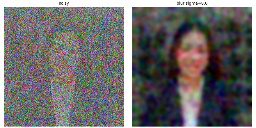
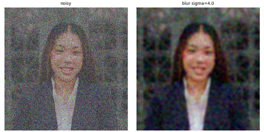
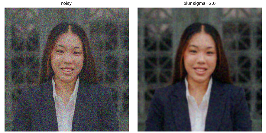
The supplied Gaussian baseline divides each noisy input by t to restore the image amplitude, then applies Gaussian blur. It tests σ = 1, 2, 4, 8, and 16 with kernel width 6σ + 1 and selects the lowest mean squared error (MSE) against the original. The selected σ values are 8, 4, and 2 at t = 0.25, 0.50, and 0.75. Blur reduces grain but loses facial detail, especially at t = 0.25.
1.3 One-step denoising
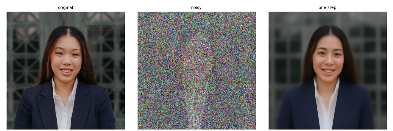
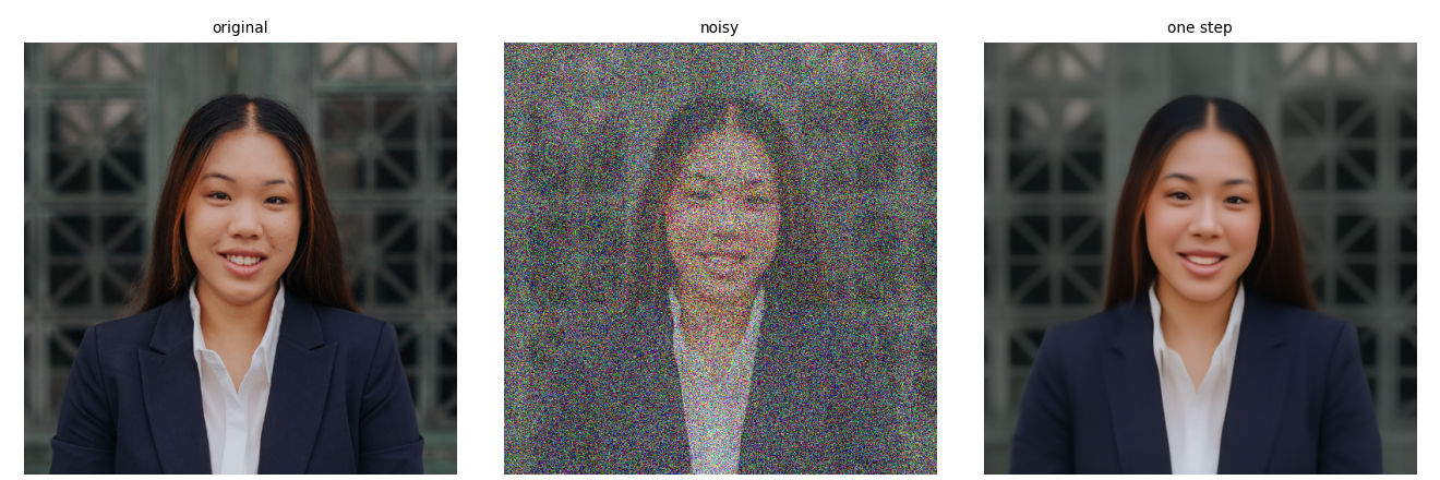
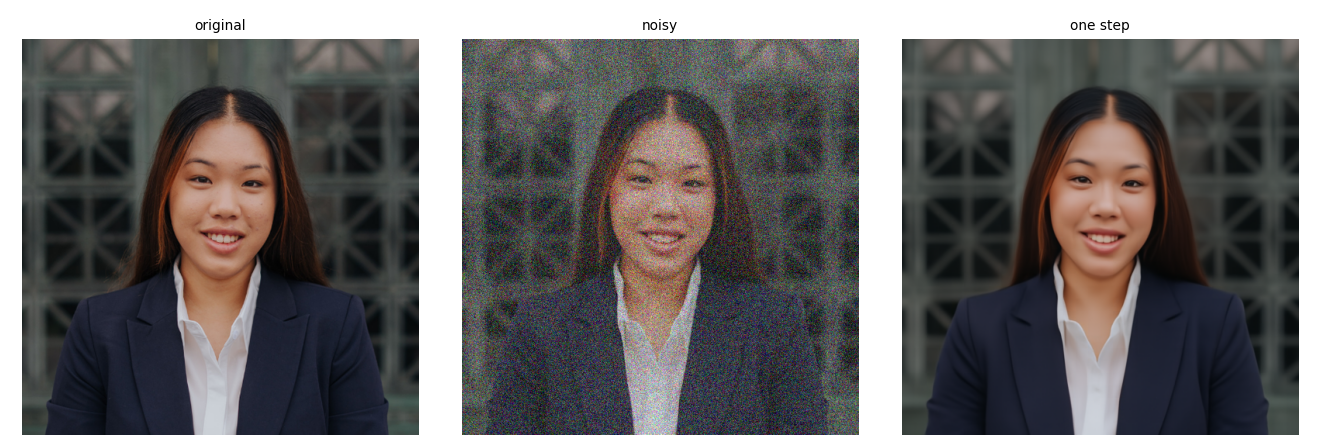
I predicted the velocity once and estimated the clean endpoint with x̂₁ = xₜ + (1 − t)vθ(xₜ, t, c), where c is the photo prompt embedding. The portrait is much clearer than the Gaussian baseline. At t = 0.25, the estimate smooths the face and background more than at t = 0.75.
1.4 Visualizing velocity
The exact velocity for this image/noise pair is x₁ − ε. I compared the predicted update (1 − t)vθ with the ground-truth update (1 − t)(x₁ − ε). For each pixel, I squared their difference, averaged over RGB, and took the square root before any display scaling. The supplied plotting code displays all updates on one symmetric RGB scale, with zero at middle gray. All error maps share one linear scale from zero to the largest error across the three times.

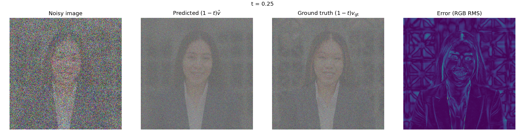
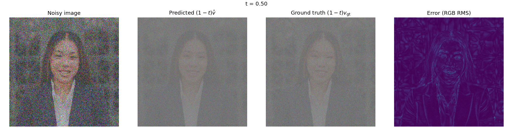
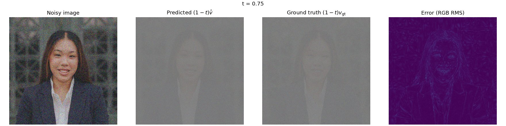
The error maps are brighter and more structured at t = 0.25. Errors remain around the face and background at t = 0.50, while the t = 0.75 map is much darker. More image information and a smaller remaining update make the later-time estimate closer to the known target.
1.5 Iterative denoising with Euler sampling
My sampler recomputes velocity after each update x ← x + hvθ(x, t, c). It shortens the last step to reach t = 1 exactly. From the saved t = 0.50 input, h = 0.02 gives 25 updates.
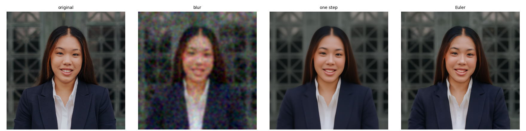
Euler sampling restores a clear portrait, but it does not have the lowest pixel error in this example. The saved reconstruction MSE is 0.00926410 for blur, 0.00212908 for one step, and 0.00250297 for Euler. Both learned methods preserve more detail than blur; one step stays slightly closer to the original by this metric.
1.6 Generating images from noise
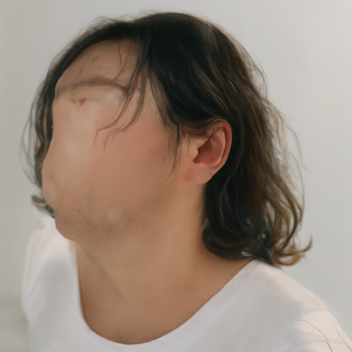
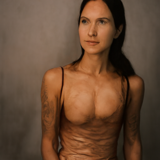
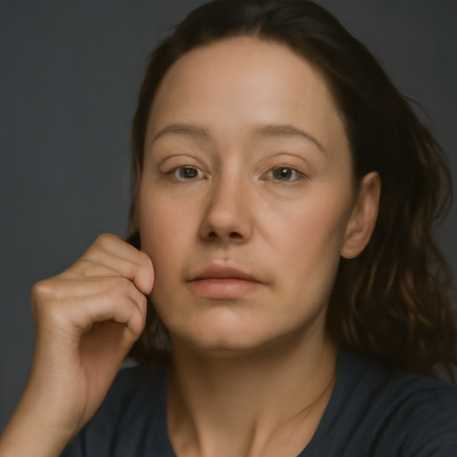
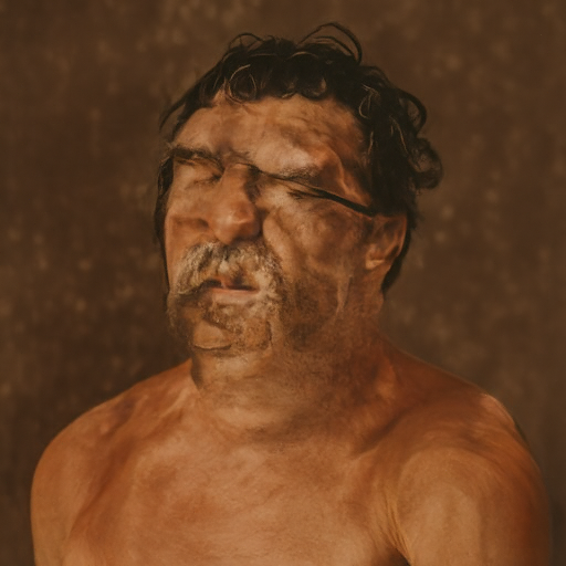
I started from five independent Gaussian tensors at t = 0 and used 50 Euler updates. Seeds 180–184 are shown in order. The generic photo prompt produces people in all five samples. Some faces and bodies are distorted; seed 183 has a particularly rough, painterly appearance.

2. Conditional generation and guidance
2.1 Classifier-free guidance (CFG)
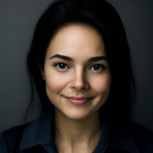
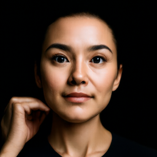
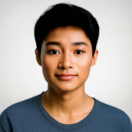
I evaluated the conditional and empty-prompt velocities at the same image and time, then used vCFG = v꜀ + w(v꜀ − vᵤ). The supplied check confirmed that w = 0 reproduces ordinary conditional prediction. The results below use w = 7 and exactly the same initial noises as above. Faces are more coherent and the outputs look more like studio portraits. These five results still concentrate on people, so this prompt gives limited subject diversity.


3. Creative applications
3.1 Image-to-image editing
I mixed each input with the same seed-180 noise at the selected starting time, then integrated to t = 1 with CFG. Every panel includes the original and all seven starts: 0.02, 0.04, 0.06, 0.10, 0.14, 0.25, and 0.50. The prompt is "a high quality photo". Smaller starting times leave less input information and allow larger changes.
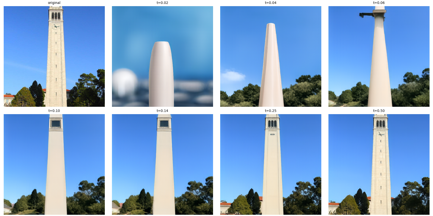
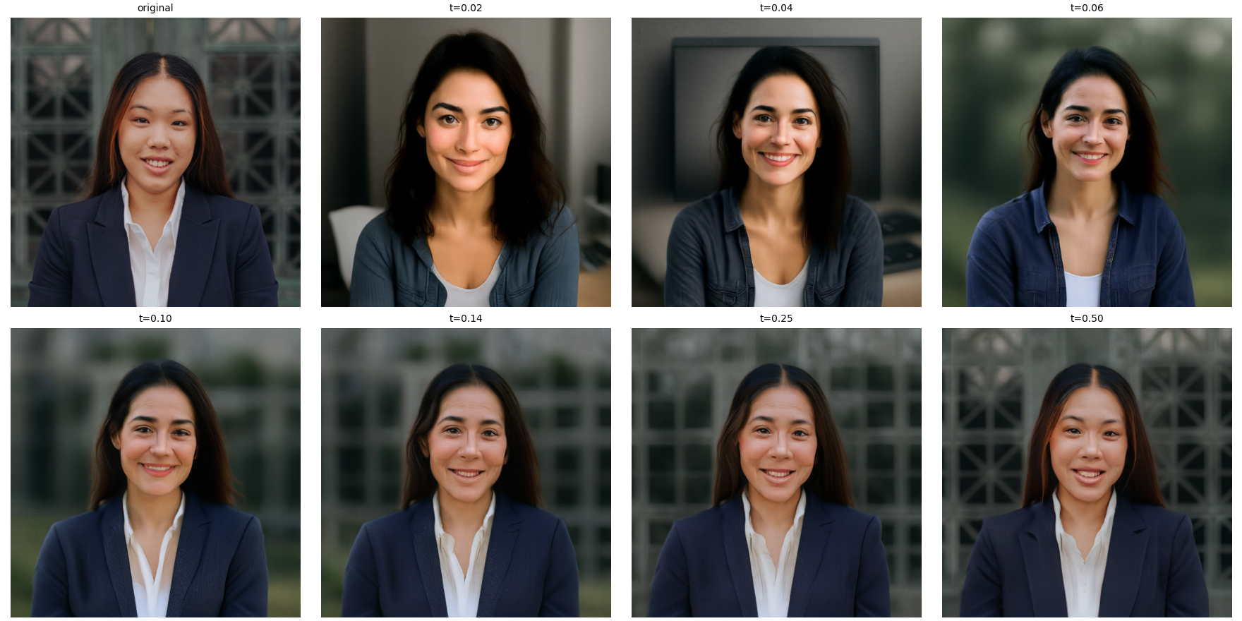

At low starting times, the Campanile becomes a smooth tower with little architectural detail, and my portrait becomes a different person. In the second test image, the smallest starts also change the subject and objects. By t = 0.25 and 0.50, the outputs stay much closer to the inputs.
Editing Hand-Drawn and Web Images
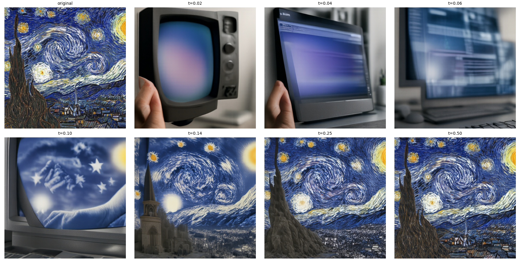
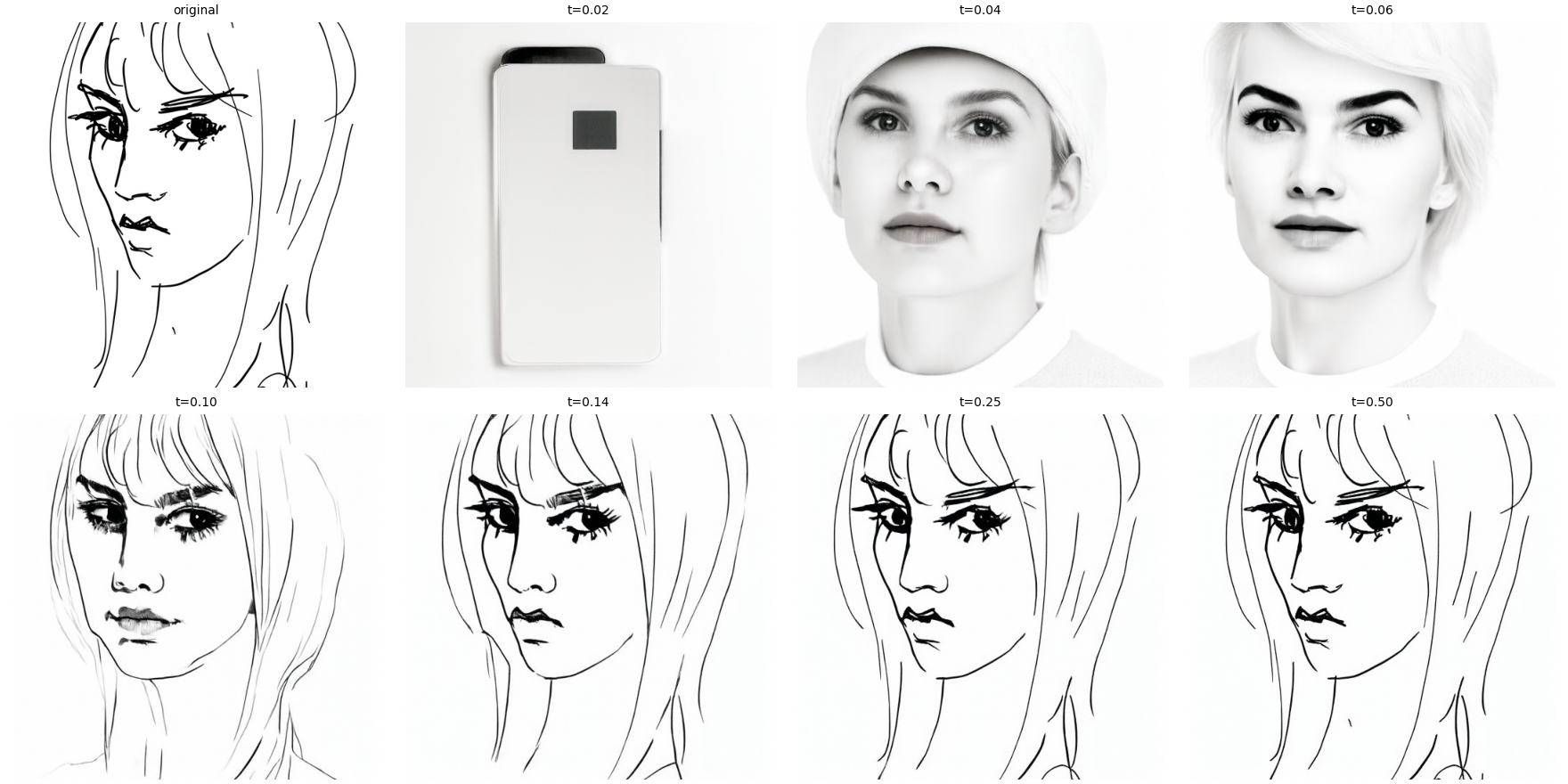
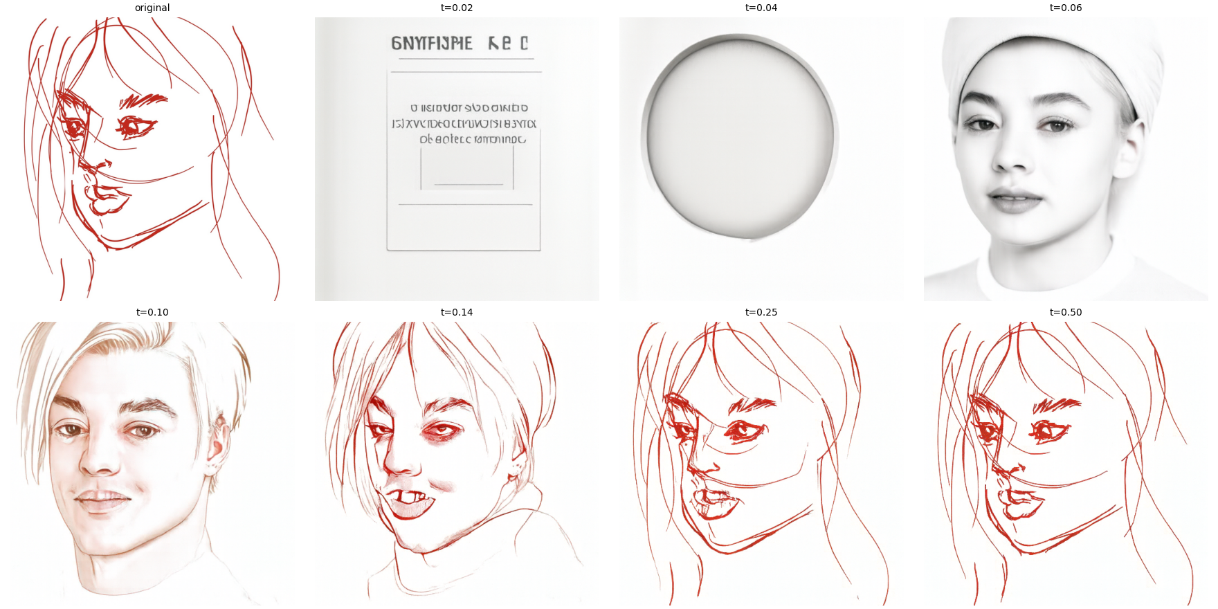
At the smallest starts, the painting becomes screens and electronic devices. Its sky and brushwork return at larger starts. The drawings can become unrelated objects at t = 0.02 or 0.04. Intermediate starts produce shaded faces, while t = 0.25 and 0.50 preserve much of the line work.
3.2 Text-guided image editing
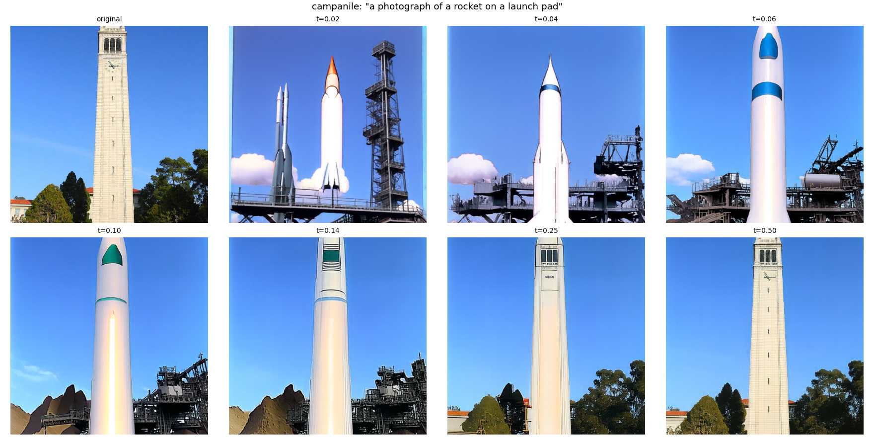
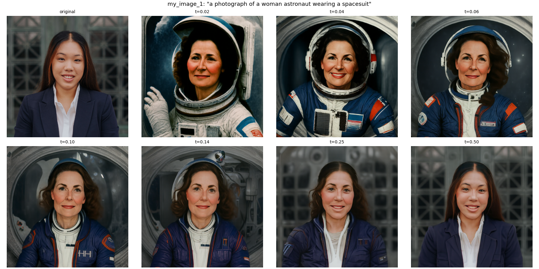
I kept the same inputs, seed, guidance weight, and seven starting times, and changed the prompt for each input.
Prompt: "a photograph of a rocket on a launch pad".
Prompt: "a photograph of a woman astronaut wearing a spacesuit".
Prompt: "an oil painting of a woman in the style of Vincent van Gogh".
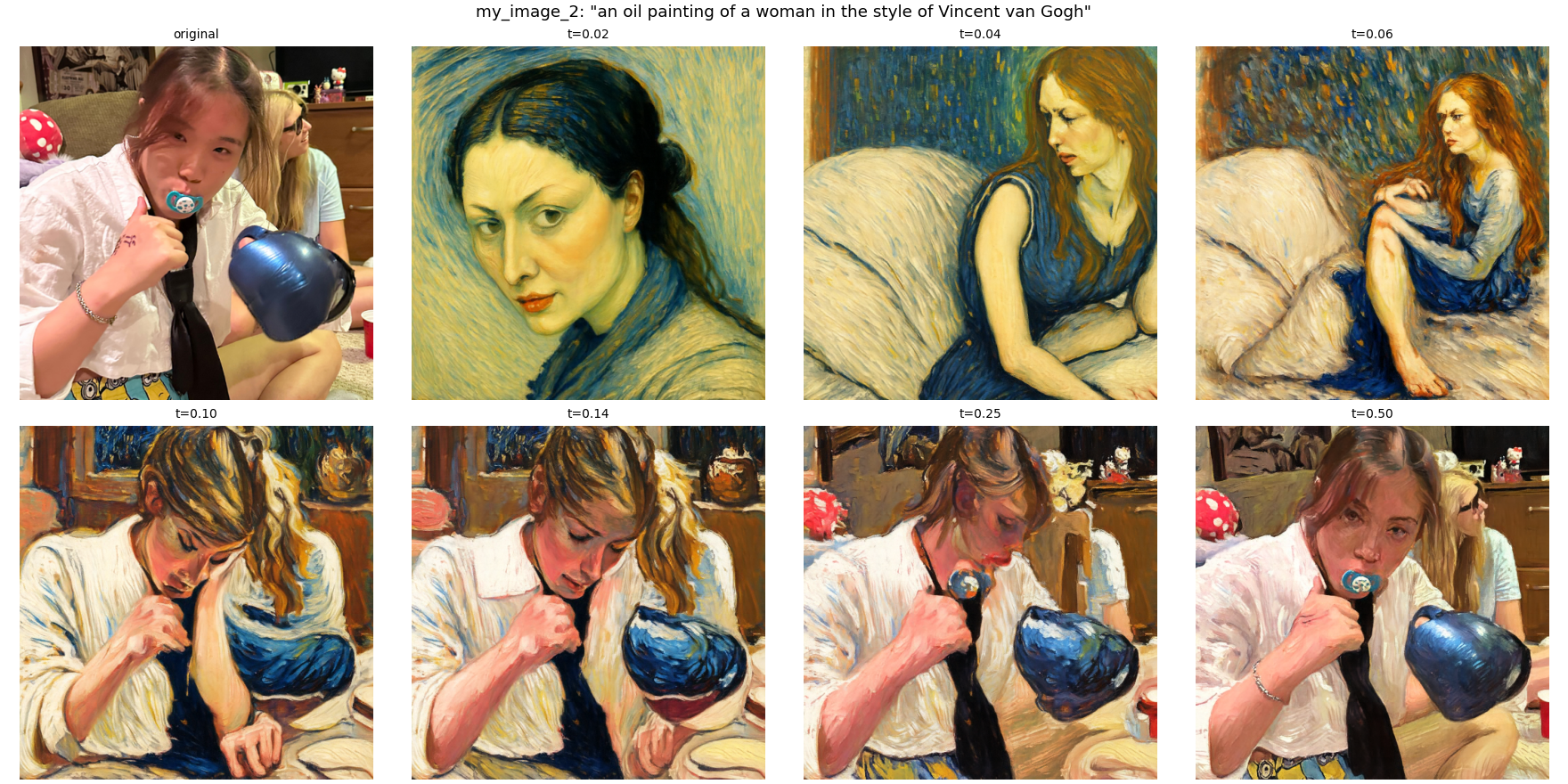
The rocket and spacesuit prompts make large changes at small starting times. At intermediate times, the rocket keeps the tower’s vertical shape and the spacesuit keeps the portrait’s framing. At t = 0.25 and 0.50, much of the original returns despite the prompt. The painting prompt adds visible painted texture to the second test image, but the smallest starts change its composition and person.
3.3 Visual anagrams
At each step, I predicted one guided velocity in the upright view and another in the view rotated 180°. I rotated the second velocity back and averaged the two before the Euler update. The supplied rotation helper flips both spatial axes and passed the supplied identity check when applied twice. I used the skeleton’s prompt pairs. These runs use seeds 180 and 181, h = 0.02, and w = 7.
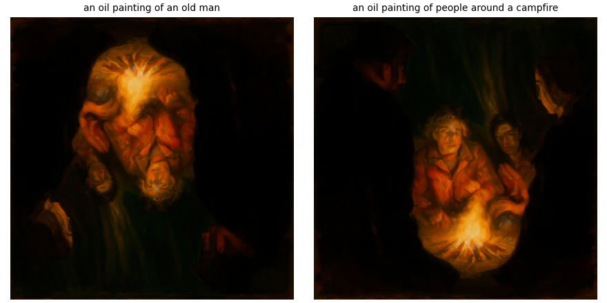
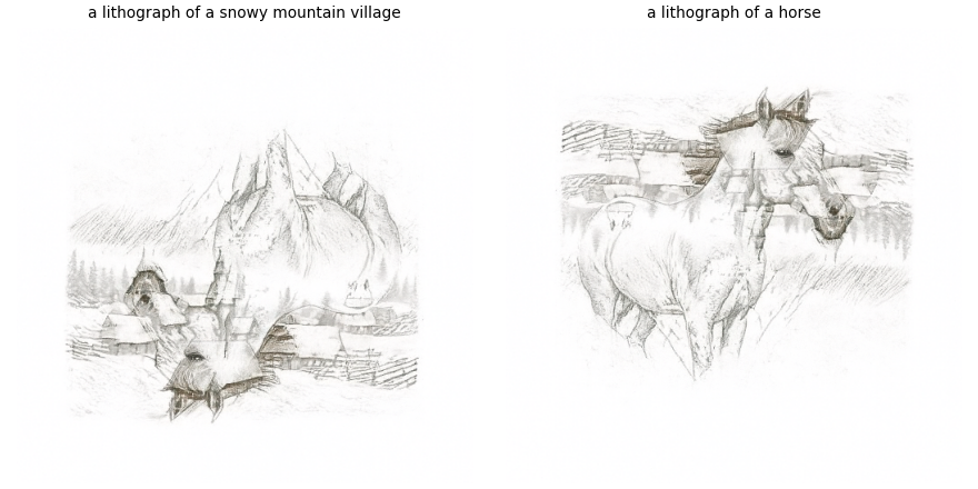
The first image has an old man’s face upright and people around a bright fire when rotated, though the facial details blend together. In the second image, the snowy mountain and buildings read upright; the rotated view has a horse’s head and body mixed with the mountain lines. The two interpretations are uneven rather than cleanly separated.
3.4 Hybrid images
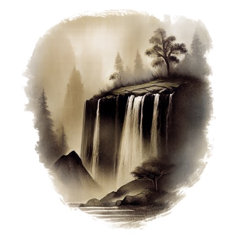
I combined the low frequencies of one CFG velocity with the high frequencies of another: v = G(vₐ) + vᵦ − G(vᵦ). I used the supplied Gaussian filter helper with kernel size 265 and σ = 16, and the skeleton’s prompt pairs. I used this combined velocity at every Euler step, with w = 7 and h = 0.02. Each pair shows a larger view beside a 64 × 64 distant view.
Distant prompt: "a lithograph of a skull". Close prompt: "a lithograph of a waterfall". Seed 180.
Distant prompt: "a lithograph of a cat". Close prompt: "a lithograph of a forest". Seed 181.
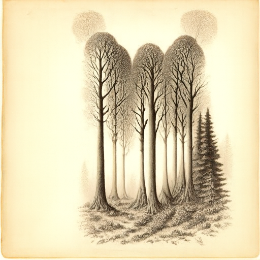
The waterfall is clear at full size, while its dark opening and broad pale shape suggest a skull at a distance. The second image clearly reads as trees nearby. Its broad canopy suggests an animal silhouette when reduced, but I do not get a clear cat face. The forest is the stronger subject in that result.
Part B: Flow matching from scratch!
The skeleton supplied the dataset and plotting helpers and the flow-matching wrapper classes. I implemented the network blocks, forward passes, losses, samplers, and experiment code.
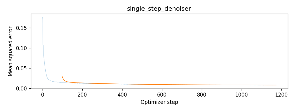
I trained on the 60,000 MNIST training images and used the 10,000-image test split for denoising examples. Pixels are in [0, 1]. Training batches are shuffled, with fresh noise drawn after each batch is fetched. The seed is 180. The loss plots show per-step MSE and a 100-step moving average.
1. Training a single-step denoising UNet
1.1 Implementing the UNet
I use D for the base number of hidden feature channels. I built convolution blocks from 3 × 3 convolutions, batch normalization, and GELU. Stride-2 convolutions reduce 28 × 28 inputs to 14 × 14 and then 7 × 7. Average pooling compresses the 7 × 7 features to 1 × 1; a transposed convolution expands them again. Upsampling blocks use transposed convolutions and concatenate features from matching encoder resolutions. A final convolution predicts one value per pixel with no output activation.
1.2 Using the UNet to train a denoiser
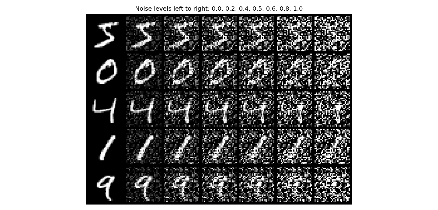
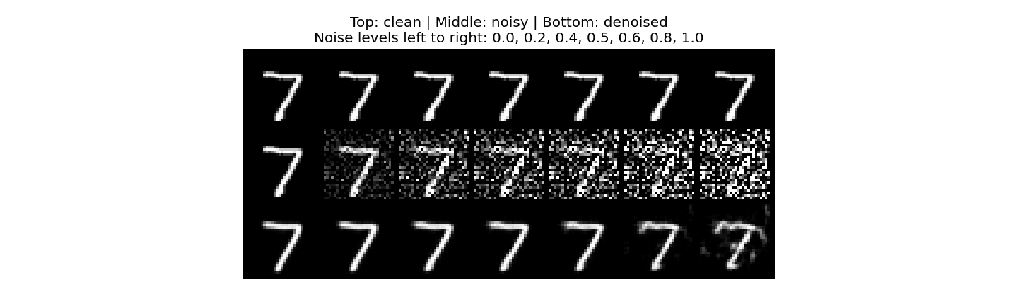
For five fixed training digits, I reused each digit’s noise pattern and formed z = x + σε at σ = 0.0, 0.2, 0.4, 0.5, 0.6, 0.8, and 1.0. This adds noise without scaling down the clean digit.
1.2.1 Training
I completed the supplied training loop with fresh noisy inputs and model predictions, and added evaluation figures and checkpoint saving. I trained a D = 128 UNet for five epochs with batch size 256, Adam learning rate 0.0001, and σ = 0.5. The MSE target is the clean image. I kept ten test digits and their noise fixed across the epoch comparisons. Mean training loss falls from 0.020177 in epoch 1 to 0.008300 in epoch 5.
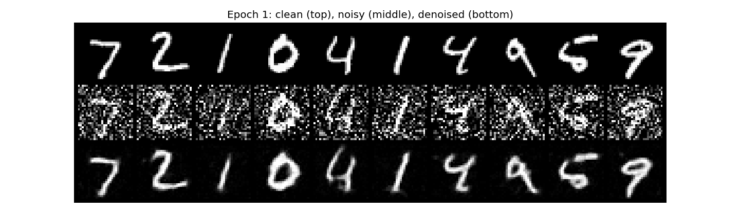
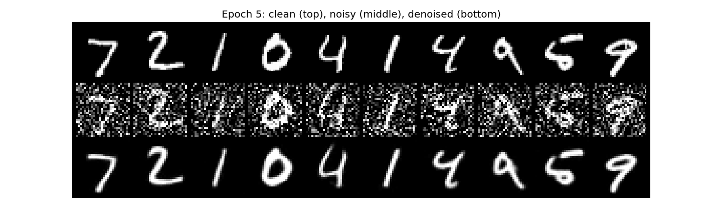
The epoch 1 predictions already recover most digit shapes. At epoch 5, strokes are cleaner and small breaks are reduced. Some fine features are still smoothed.
1.2.2 Out-of-distribution testing
I kept the same test digit and Gaussian noise pattern and varied σ across the seven levels. The model was trained only at σ = 0.5. It retains the 7 at lower noise levels, but the stroke becomes less stable at σ = 0.8 and 1.0. The highest-noise output has extra marks and a less clear shape.
1.2.3 Denoising pure noise
I trained a fresh D = 128 UNet for five epochs with the same batch size, Adam learning rate, and MSE objective, but gave it independent Gaussian noise as input and a clean digit as target. The ten evaluation noise inputs stay fixed. Mean training loss is 0.073273 in epoch 1 and 0.067408 in epoch 5.
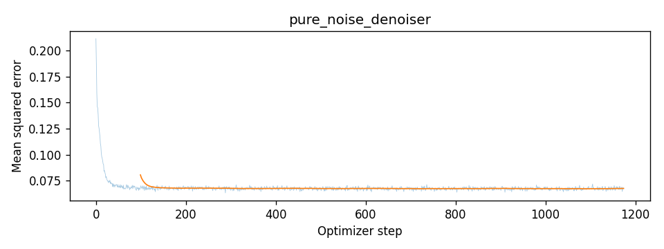


Different noise inputs produce nearly identical blurry outputs. Their bright centers and overlapping curves resemble an average of the training digits. Since the input noise is independent of the target, it gives the model no information about which digit to predict. Under MSE, predicting the conditional mean minimizes expected error; here that mean is the average training image. A lower loss therefore does not imply varied, recognizable generated digits.
2. Training a flow matching model
2.1 Adding time conditioning to UNet
I added two FCBlocks, each with Linear → GELU → Linear, to embed normalized time. Their outputs multiply features after unflattening and after the first upsampling block.
2.2 Training the UNet
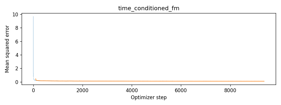
For each training image x₁, I sample Gaussian x₀ and t uniformly in [0, 1], form xₜ = (1 − t)x₀ + tx₁, and train the UNet to predict x₁ − x₀ using MSE.
This D = 64 model uses batch size 64 and Adam with initial learning rate 0.01 for ten epochs. After each epoch, the exponential scheduler multiplies the learning rate by 0.1^(1/10), about 0.7943. Mean training loss decreases from 0.185022 in epoch 1 to 0.093514 in epoch 10.
2.3 Sampling from the UNet
Sampling uses 50 Euler steps of size 0.02 from pure noise. I reuse seeds 180–189 at all three checkpoints.



Epoch 1 contains scattered strokes and ambiguous shapes. By epochs 5 and 10, more outputs resemble digits, including several clear 3, 6, 7, and 9 shapes. Some epoch 10 outputs remain broken or malformed. Time conditioning improves generation, but this run does not produce ten clean digits.
2.4 Adding class-conditioning to UNet
I represented each digit label as a ten-element one-hot vector and added two class FCBlocks. At two decoder stages, I use class_embedding × features + time_embedding.
2.5 Training the UNet
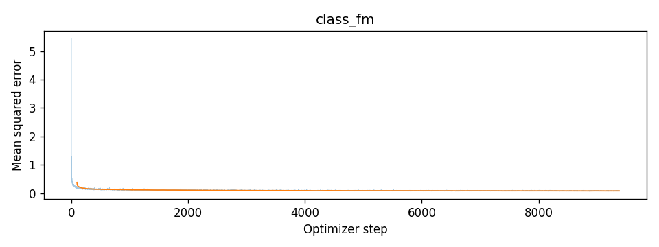
During training, I zero the entire class vector with probability 0.1 before embedding it, so the same model can predict an unconditional velocity.
I trained a fresh D = 64 model for ten epochs with batch size 64, Adam initial learning rate 0.01, and the same exponential decay.
2.6 Sampling from the UNet
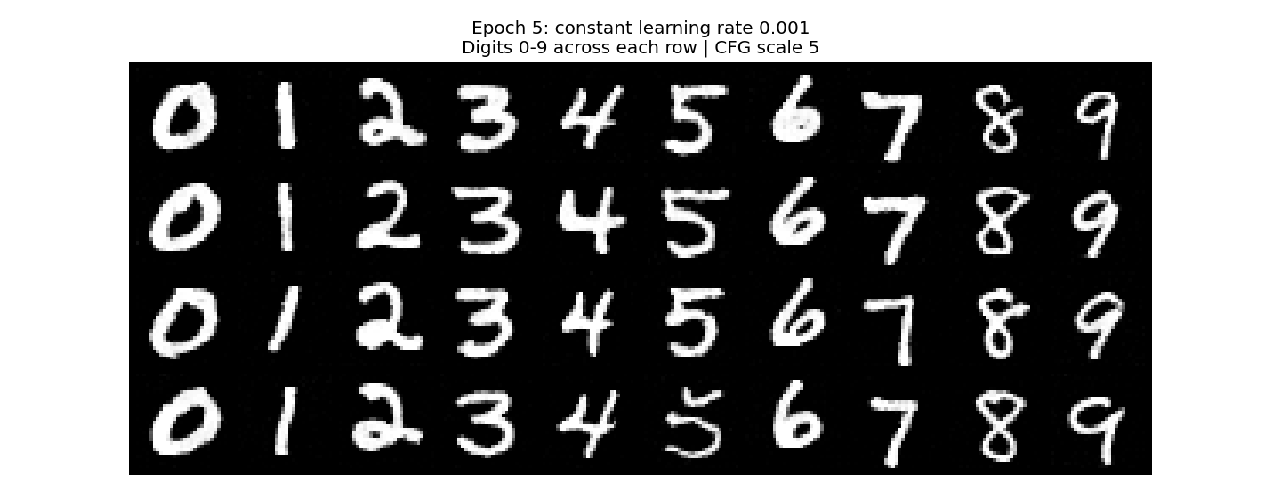
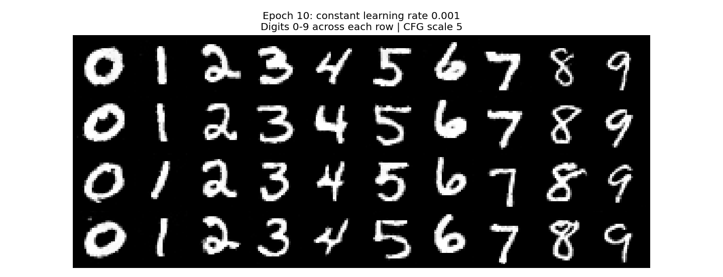
Sampling uses 300 Euler steps, h = 1/300, and v = vᵤ + 5(v꜀ − vᵤ). This Part B guidance convention differs from Part A’s v꜀ + w(v꜀ − vᵤ). Each grid requests digits 0–9 across four rows, with sampling seed 180 held fixed across epochs.
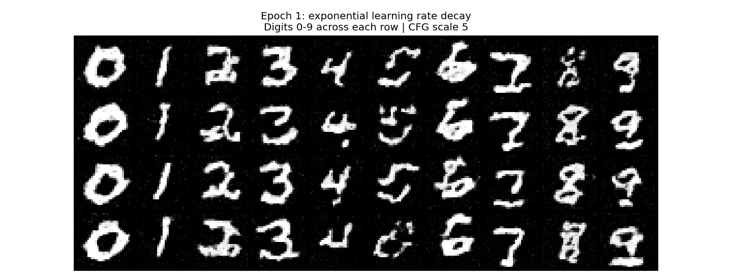
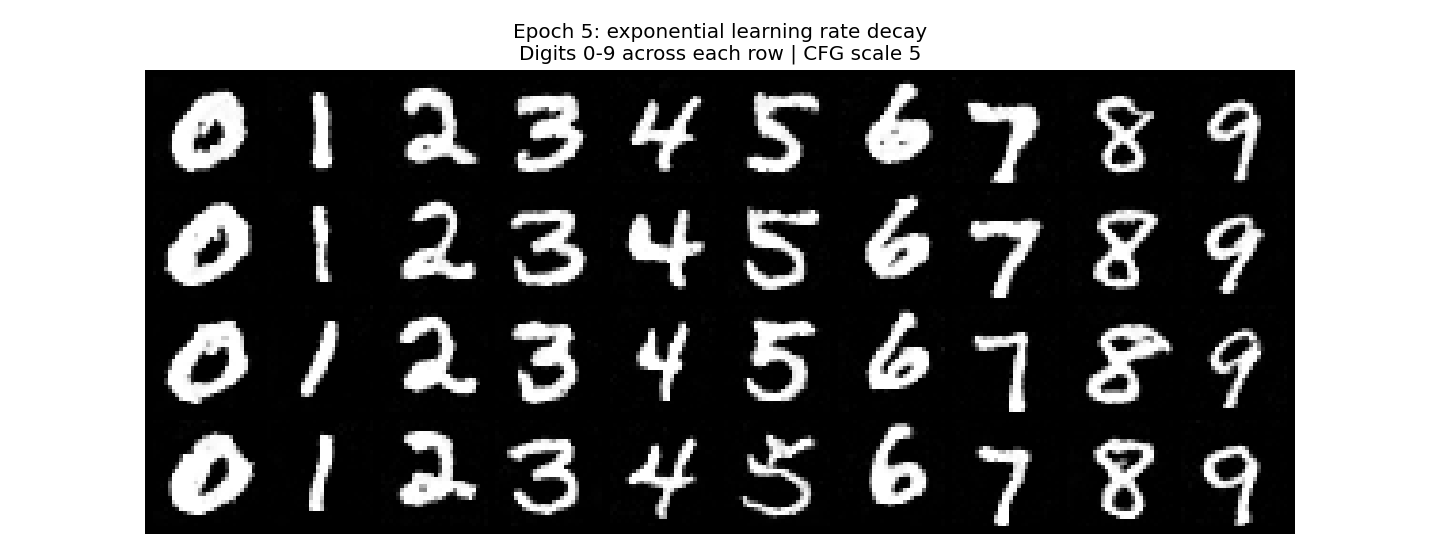
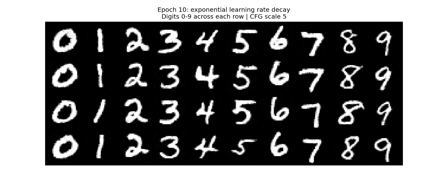
Epoch 1 already follows many requested labels, but several digits are rough or fragmented. By epochs 5 and 10, the requested digits are recognizable, with variation in tilt, stroke width, and loop shape. Class conditioning gives more consistent digit shapes than the time-only model in these samples.
Removing the learning rate scheduler
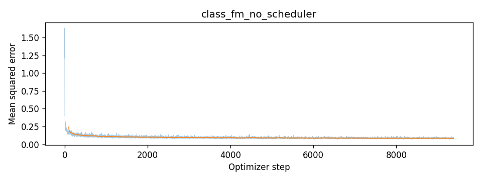
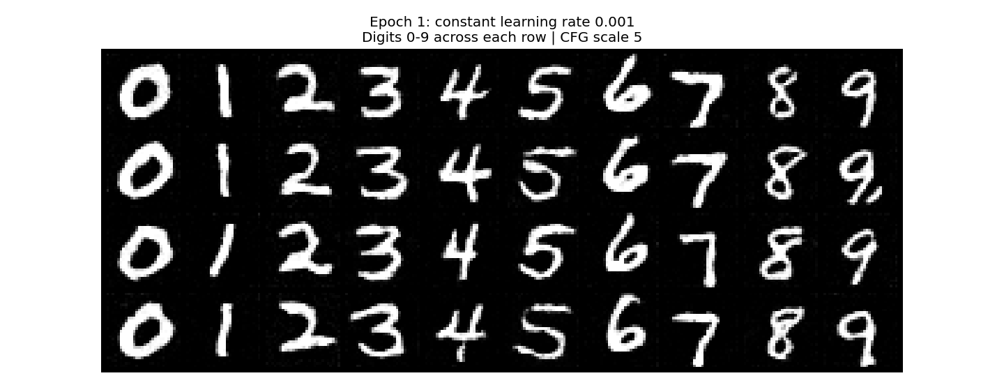
I trained an independent model with a constant learning rate of 0.001. I lowered the initial rate from 0.01 to compensate for removing decay; 0.001 is also the scheduled run’s rate after ten decay steps. I kept the architecture, epochs, batch size, class dropout, and sampling settings the same. Both experiments reset the training seed and data-loader seed to 180, and use the same initial sampling noise.
| Epoch | Exponential decay | Constant 0.001 |
|---|---|---|
| 1 | 0.169910 | 0.136794 |
| 5 | 0.093312 | 0.091006 |
| 10 | 0.084713 | 0.085003 |
The constant-rate model looks cleaner at epoch 1 and has a lower mean training loss. By epoch 10, both produce recognizable requested digits and their mean losses are close. In this experiment, reducing the constant learning rate maintained similar final performance without a scheduler.