Project 4: [Auto]Stitching Photo Mosaics
Part A: Image Warping and Mosaicing
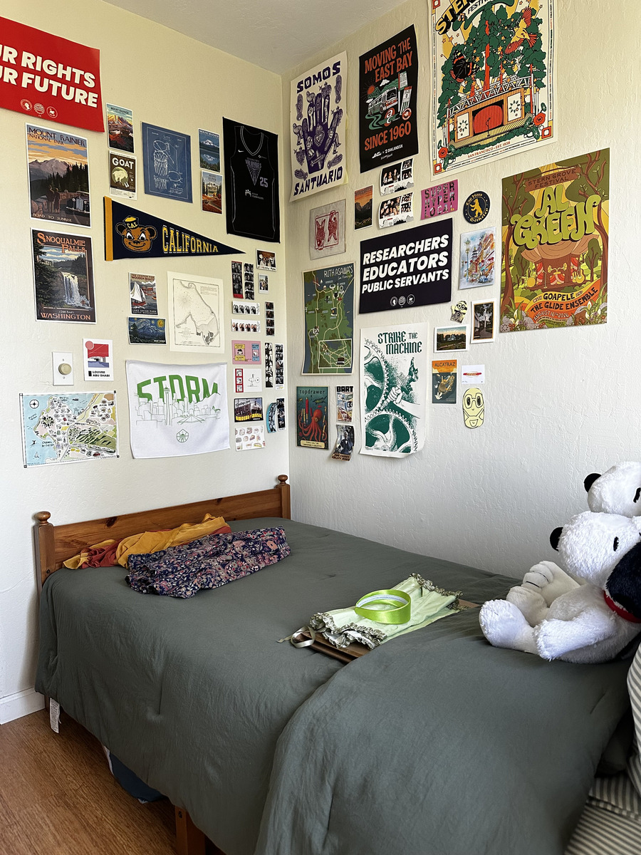
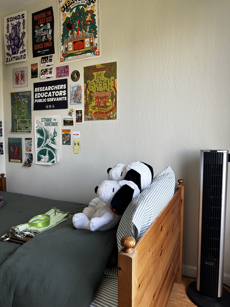
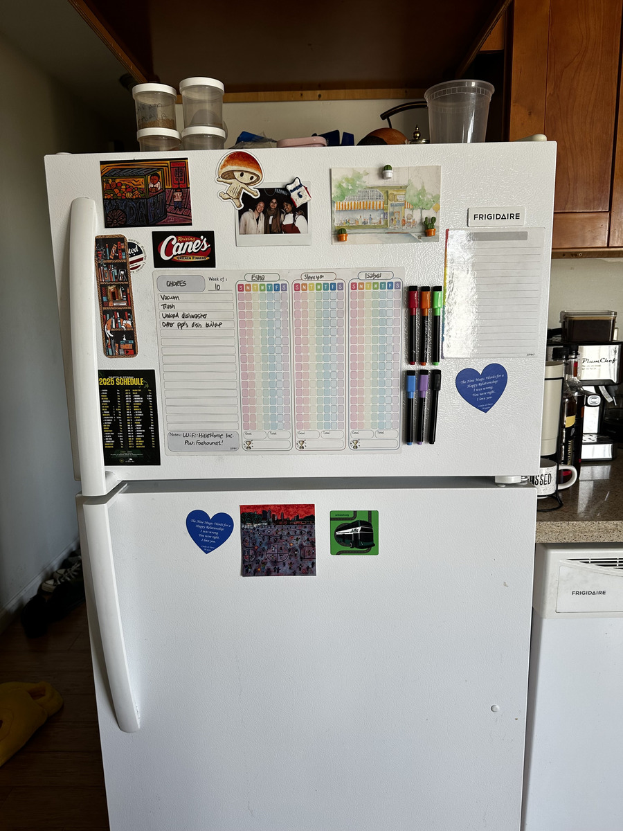
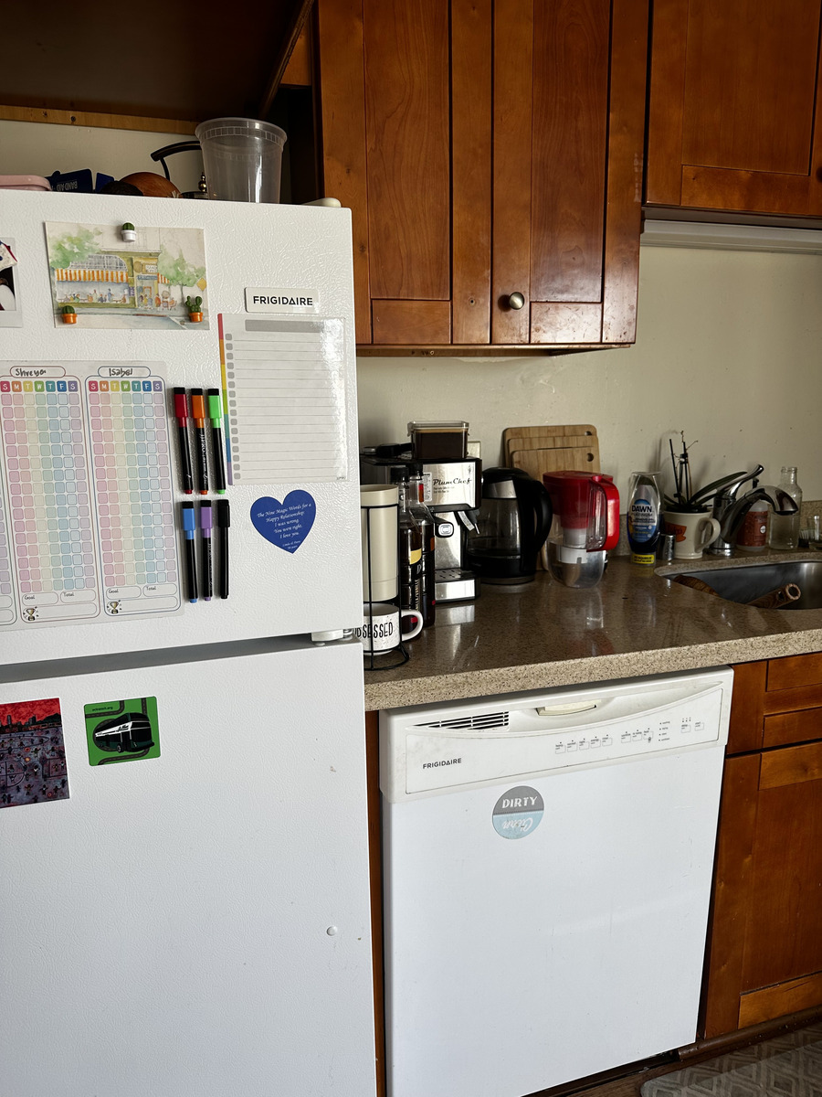
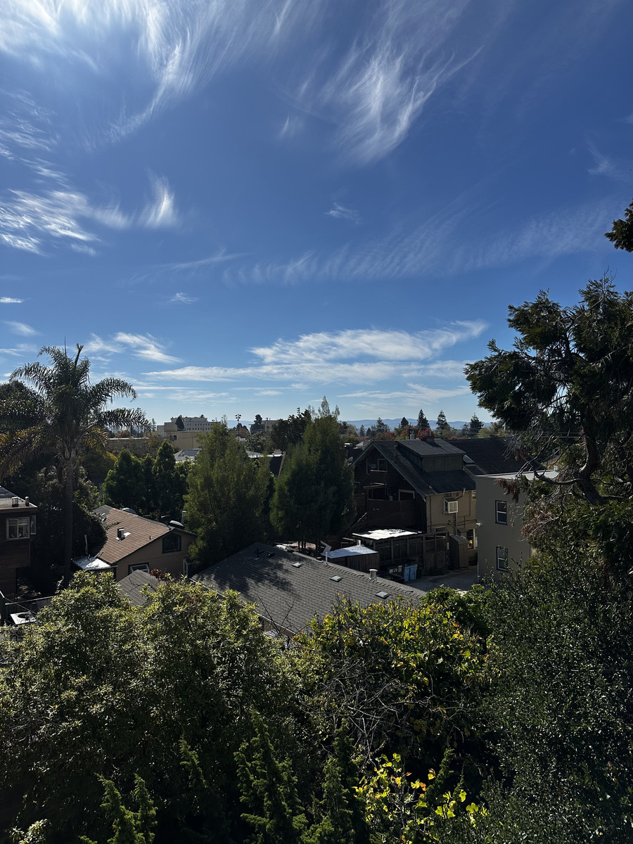
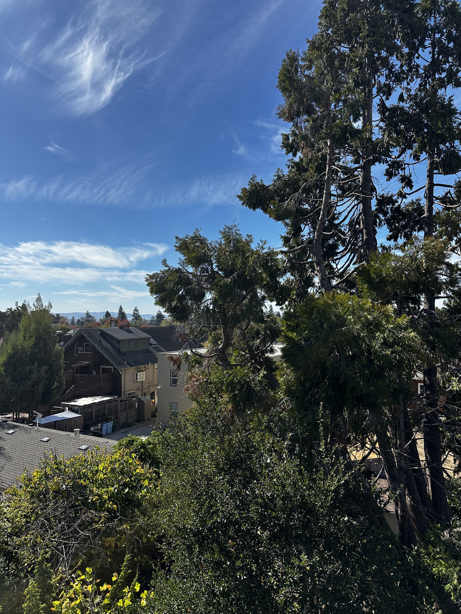
I estimated homographies from manually selected points, implemented inverse warping with nearest-neighbor and bilinear interpolation, and blended overlapping photos into mosaics. The images show my bedroom, kitchen, and the view outside my apartment.
A.1: Shoot the Pictures
I took two overlapping views of each scene. For matching points, I used poster corners in the bedroom, details on the fridge in the kitchen, and building corners outside.
Bedroom
Kitchen
Outdoors
A.2: Recover Homographies
I selected corresponding points with the correspondence tool and saved their (x, y) coordinates in JSON files. I applied the photos’ EXIF orientation when loading them so the arrays matched the upright images used for point selection.
A homography maps a source point (x, y) to a destination point (x′, y′). I fix the bottom-right entry at 1, which leaves eight unknown entries:
    [x′]   [h₁ h₂ h₃] [x]
  w [y′] = [h₄ h₅ h₆] [y]
    [ 1]   [h₇ h₈  1] [1]

w = h₇x + h₈y + 1
Substituting w into the first two rows gives two linear equations per point pair:
[x y 1 0 0 0 −xx′ −yx′]             [x′]
[0 0 0 x y 1 −xy′ −yy′] h =         [y′]

h = [h₁ h₂ h₃ h₄ h₅ h₆ h₇ h₈]ᵀ
I stack these rows into Ah = b. With n pairs, A has 2n rows and eight columns. More than four pairs give an overdetermined system, which I solve with np.linalg.lstsq.
Bedroom
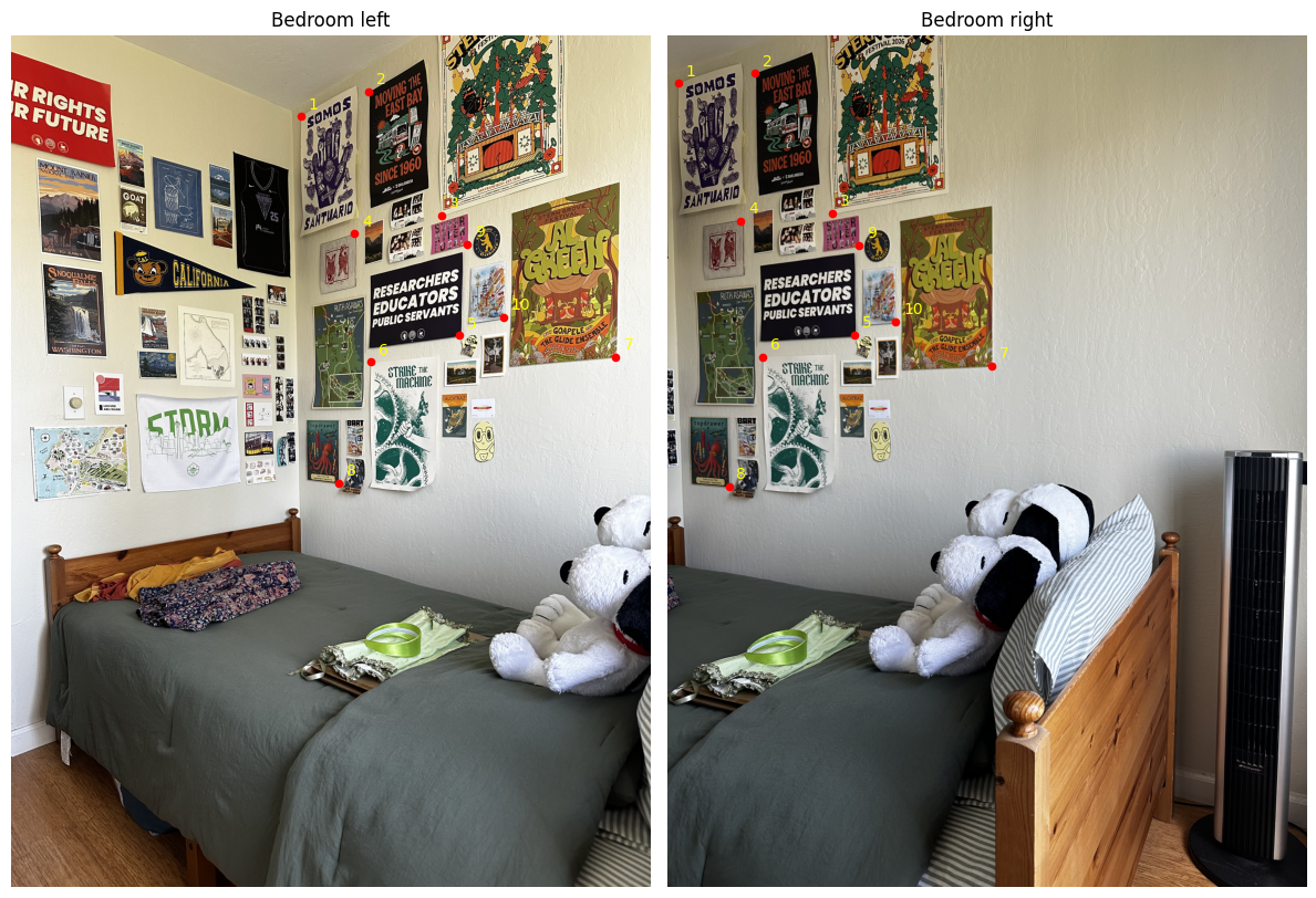
Homography from the left image to the right image:
[[ 1.49422036e+00  2.32368398e-02 -1.99178483e+03]
 [ 3.54829082e-01  1.35543482e+00 -7.25478647e+02]
 [ 1.81716269e-04 -8.79873323e-06  1.00000000e+00]]
I initially used 12 pairs, including points on the bed and stuffed animal. The mean projection error was 20.08 pixels. Keeping the ten wall points reduced it to 3.94 pixels. This is consistent with parallax from camera movement: the nearer objects and the wall do not share the same mapping.
Kitchen
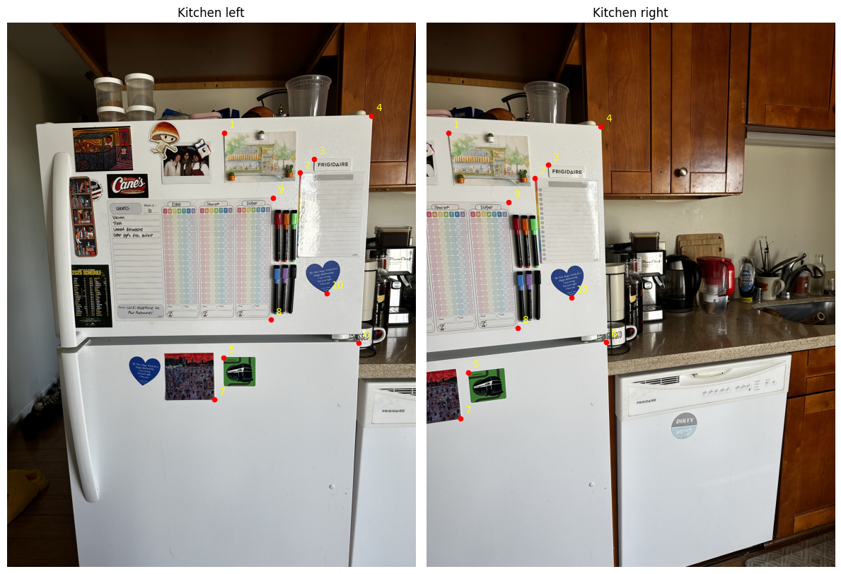
Homography from the left image to the right image:
[[ 1.48352454e+00  1.13840828e-01 -2.27450463e+03]
 [ 2.14911730e-01  1.33667949e+00 -4.26220216e+02]
 [ 1.47060454e-04  5.30656544e-06  1.00000000e+00]]
Outdoors
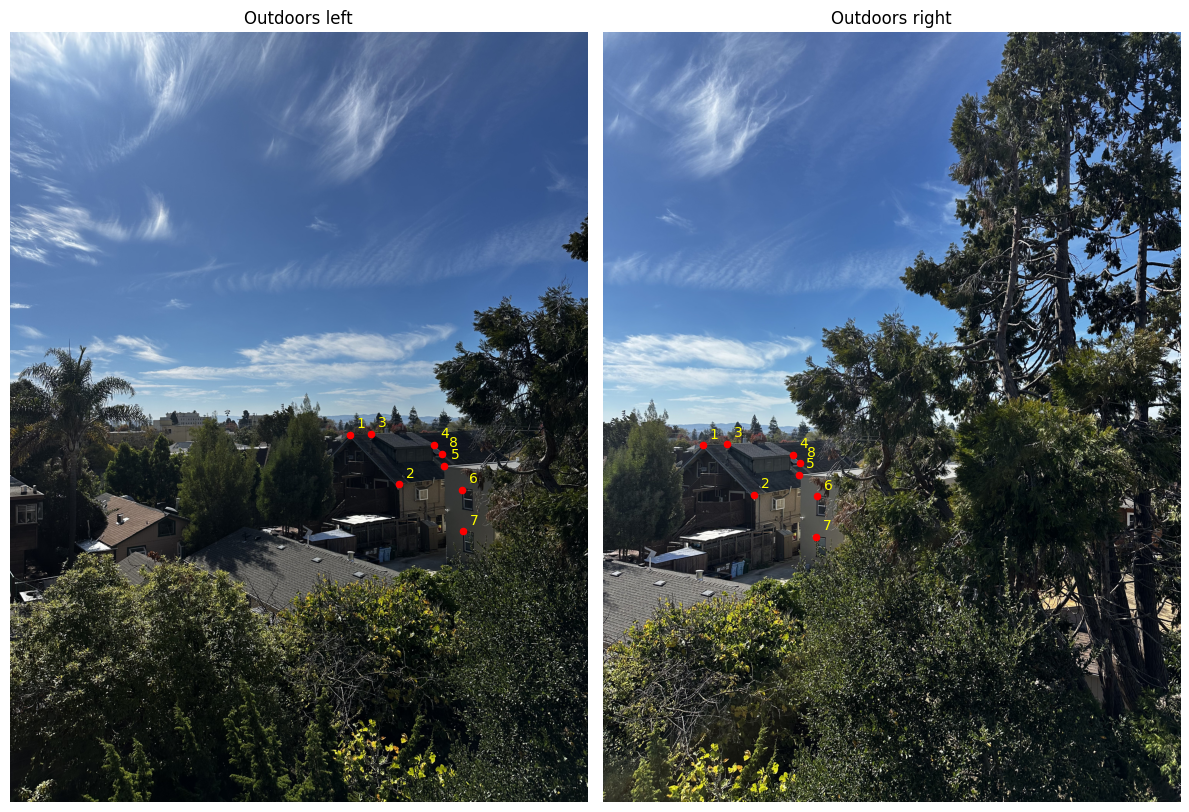
Homography from the left image to the right image:
[[ 1.67207849e+00 -2.04639720e-01 -1.87115438e+03]
 [ 6.55156604e-01  1.06313001e+00 -6.37402509e+02]
 [ 3.02983268e-04 -1.22509232e-04  1.00000000e+00]]
The eight points cover a small region around the buildings. Their fit does not establish accuracy across the sky or foreground.
| Scene | Pairs | Mean Error | Maximum Error |
|---|---|---|---|
| Bedroom | 10 | 3.94 | 7.19 |
| Kitchen | 10 | 3.95 | 8.01 |
| Outdoors | 8 | 2.33 | 4.55 |
A.3: Warp the Images
I transform the four image corners with H, round the bounds outward, and create an output pixel grid. For each output pixel, I apply H⁻¹ and divide by the homogeneous coordinate to find its position in the source image. This inverse mapping avoids holes between forward-mapped source pixels. I keep a separate validity mask for pixels whose source coordinates fall inside the image.
Nearest-neighbor interpolation rounds each valid source coordinate and copies that pixel. Bilinear interpolation uses the fractional distances dx and dy to weight the four neighboring pixels:
I(x, y) = (1 − dx)(1 − dy) I(x₀, y₀)
        + dx(1 − dy) I(x₁, y₀)
        + (1 − dx)dy I(x₀, y₁)
        + dx dy I(x₁, y₁)
I implemented both interpolation methods with NumPy. At the last row or column, I clamp the upper neighbor to the image boundary. Invalid output pixels remain black and have a false mask value.
For rectification, I selected four object corners with Matplotlib’s ginput in clockwise order and mapped them to a rectangle defined by hand. These are the two original photos:

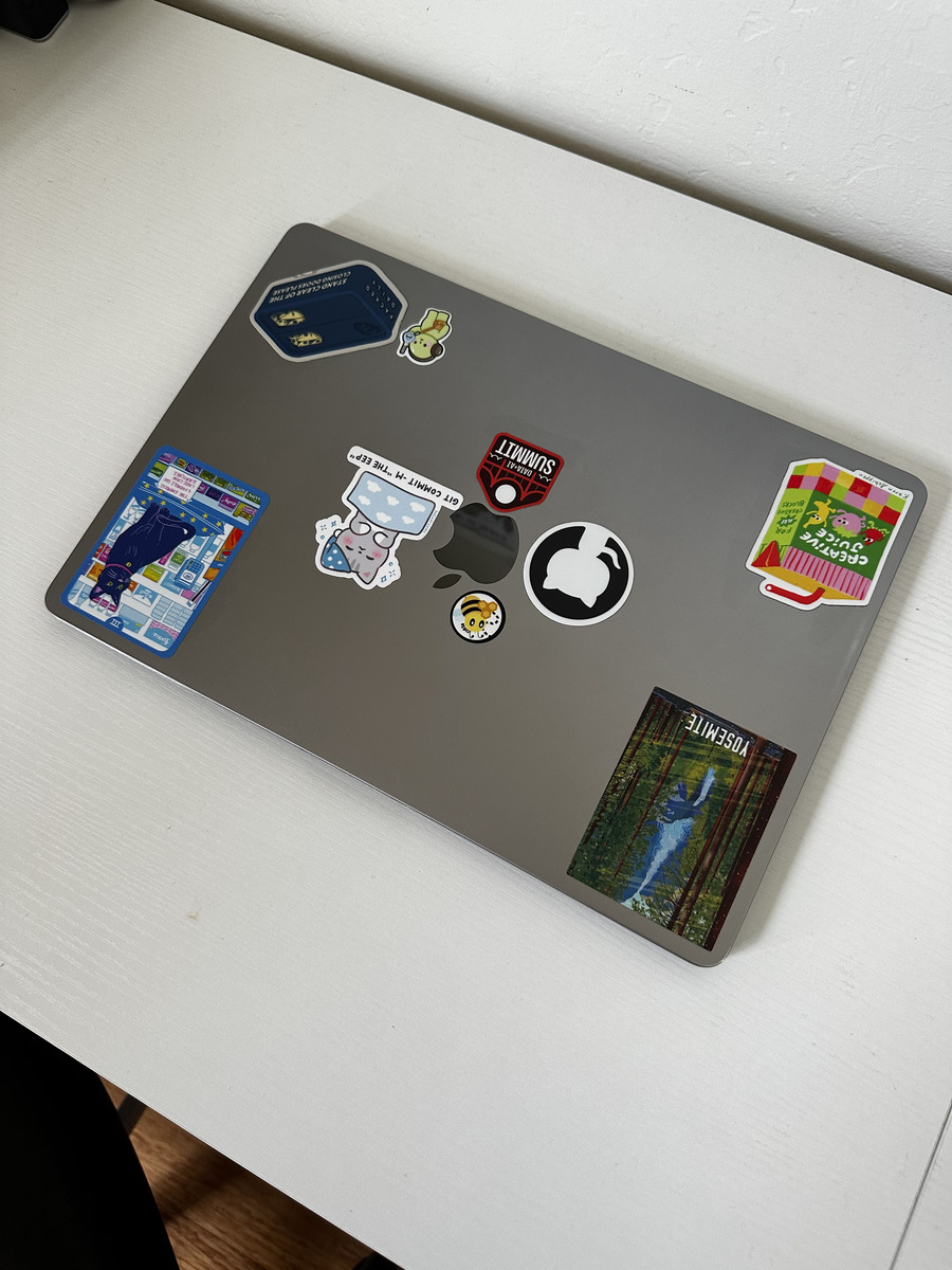
Book Rectification
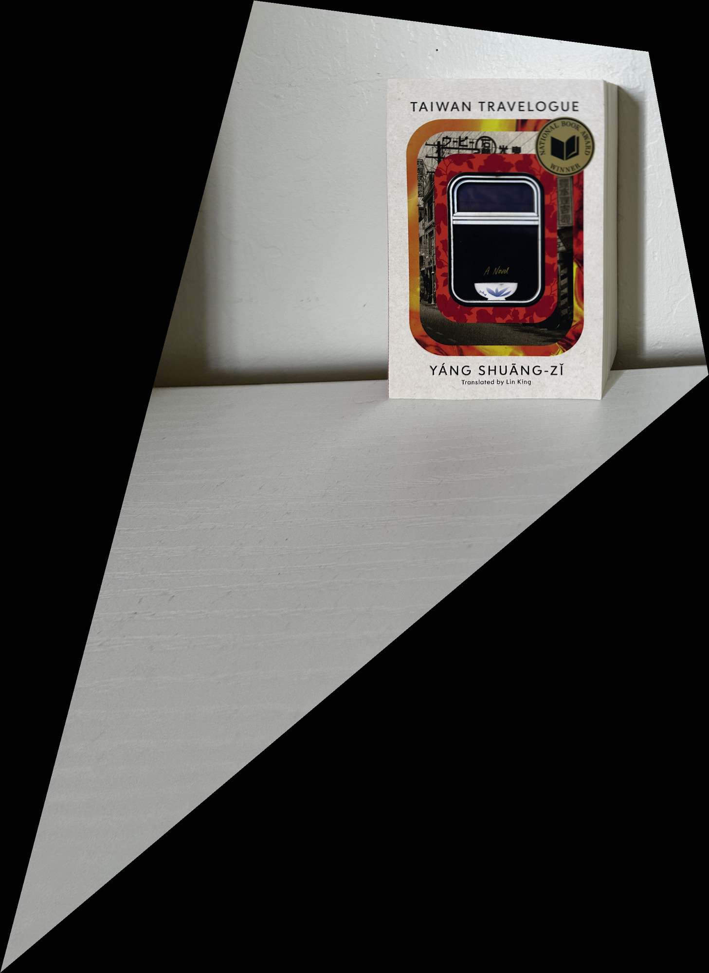
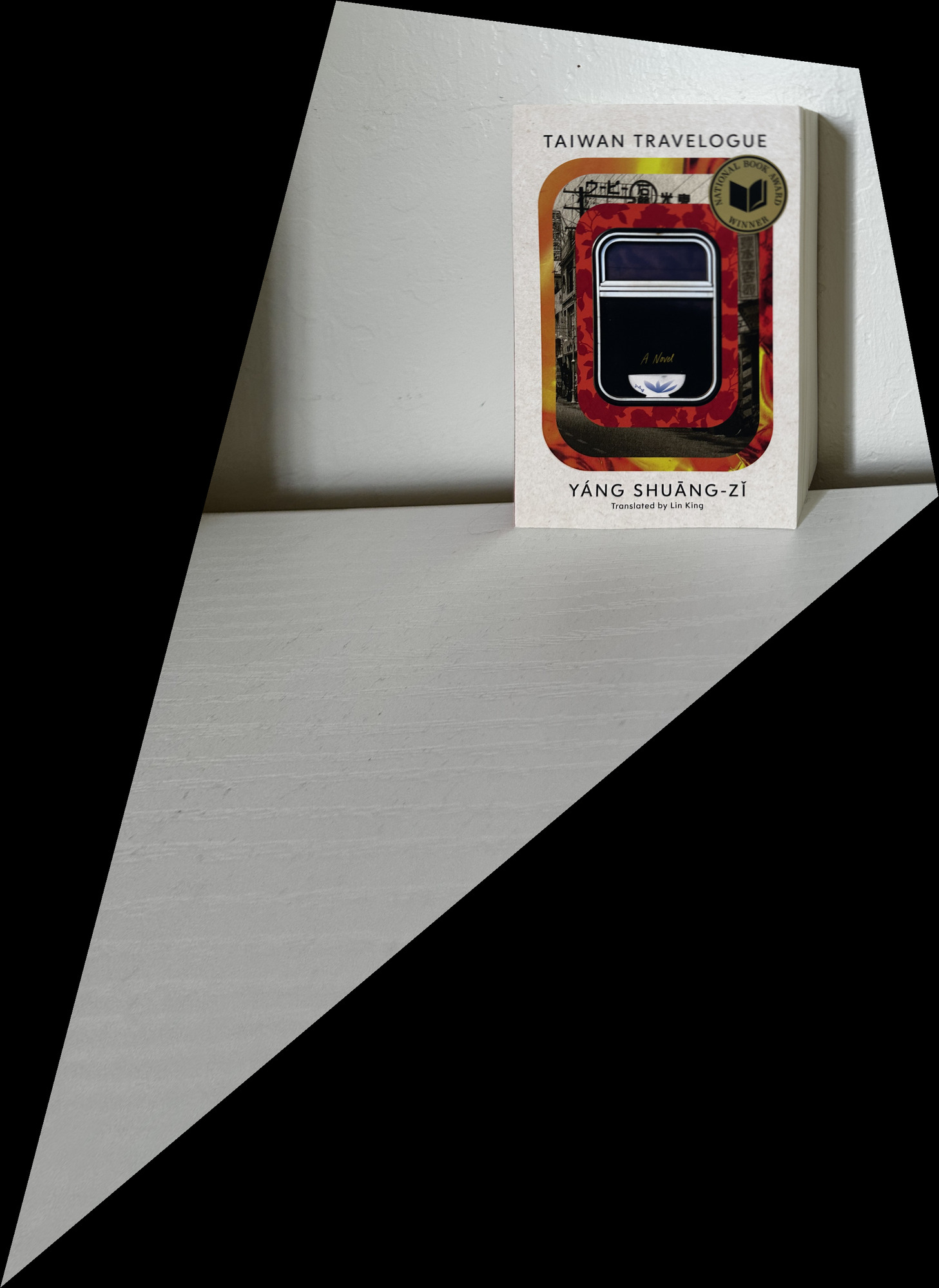
I mapped the four corners to a 600 × 900-pixel rectangle. The images below retain the full warped photo around the rectified surface.

Laptop Rectification
I mapped the four corners to a 900 × 600-pixel rectangle. The images below retain the full warped photo around the rectified surface.
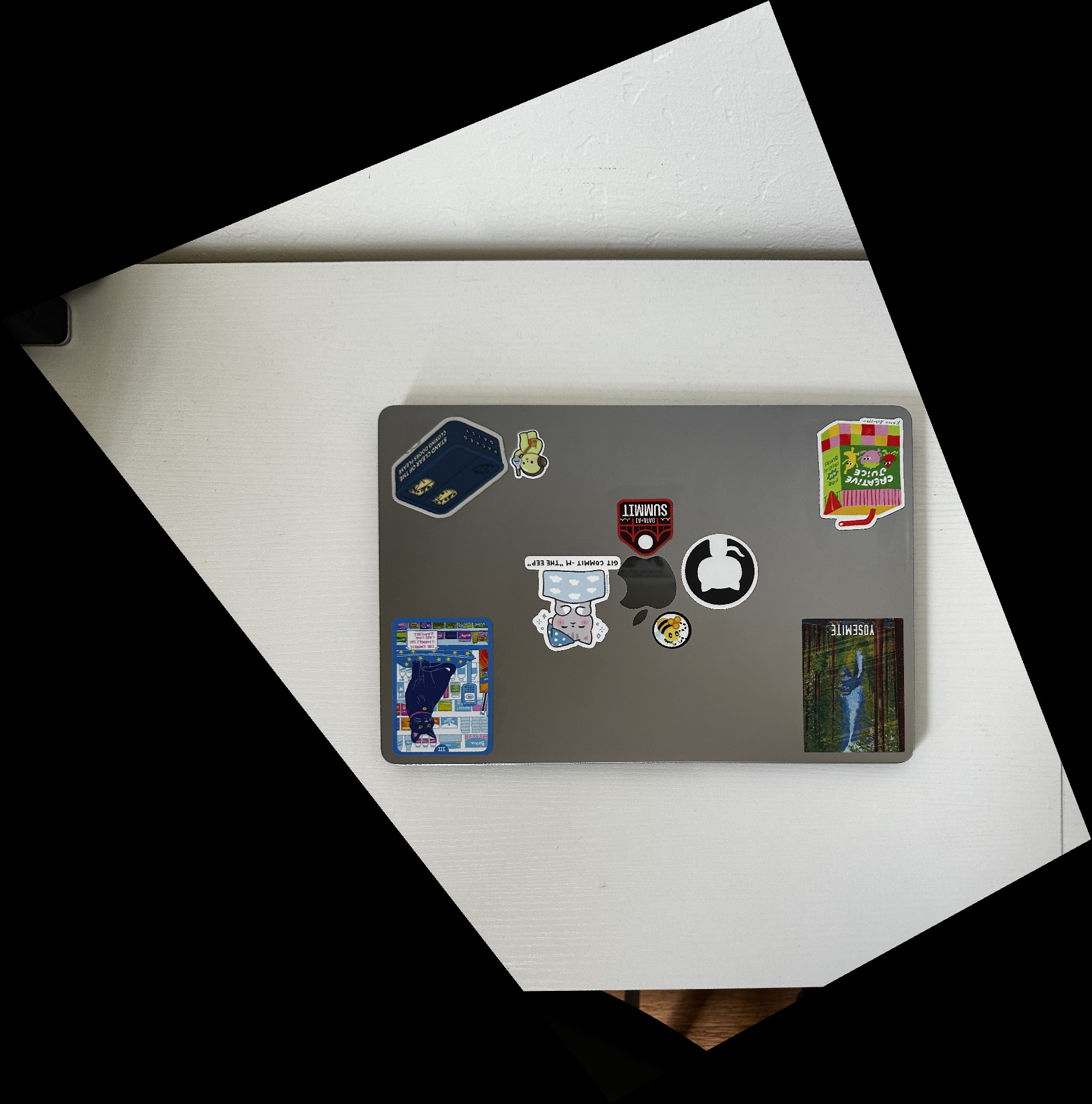
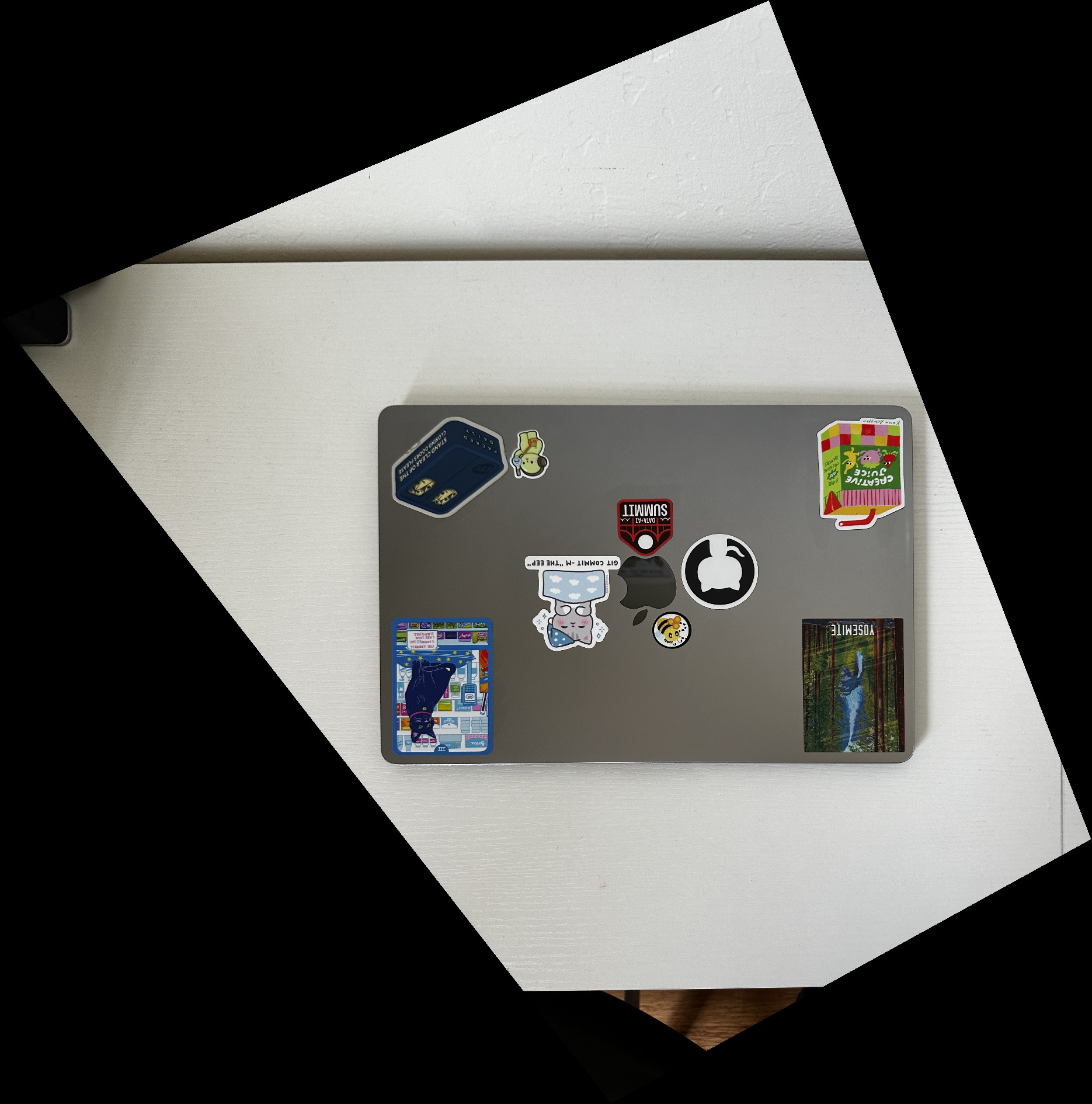
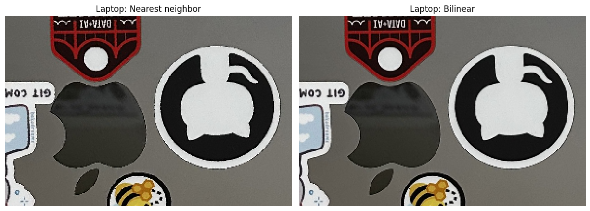
| Image | Nearest Neighbor | Bilinear |
|---|---|---|
| Book | 0.307 s | 0.528 s |
| Laptop | 0.203 s | 0.373 s |
Nearest neighbor was faster in both runs. Its text and sticker edges look more jagged in the close-ups. Bilinear interpolation gives smoother edges by averaging nearby pixels, with some loss of sharpness.
A.4: Blend the Images Into a Mosaic
For each pair, I warp the left photo into the right photo’s coordinate system with bilinear interpolation. I compute a shared canvas that contains both images, then use the warped image’s offset to place it and its validity mask. The right image stays unwarped.
I use the distance transform of each mask to set blending weights. Each mask has a one-pixel false border before the distance calculation, so the canvas edges count as image boundaries. A pixel farther from an image boundary receives more weight. If only one image covers a pixel, that image receives full weight.
w_left  = d_left  / (d_left + d_right)
w_right = d_right / (d_left + d_right)

mosaic = w_left · left + w_right · right
Where both distances are zero, I leave the output black. The masks record valid image coverage separately from pixel color, so valid black pixels still contribute to the blend.
Bedroom Mosaic
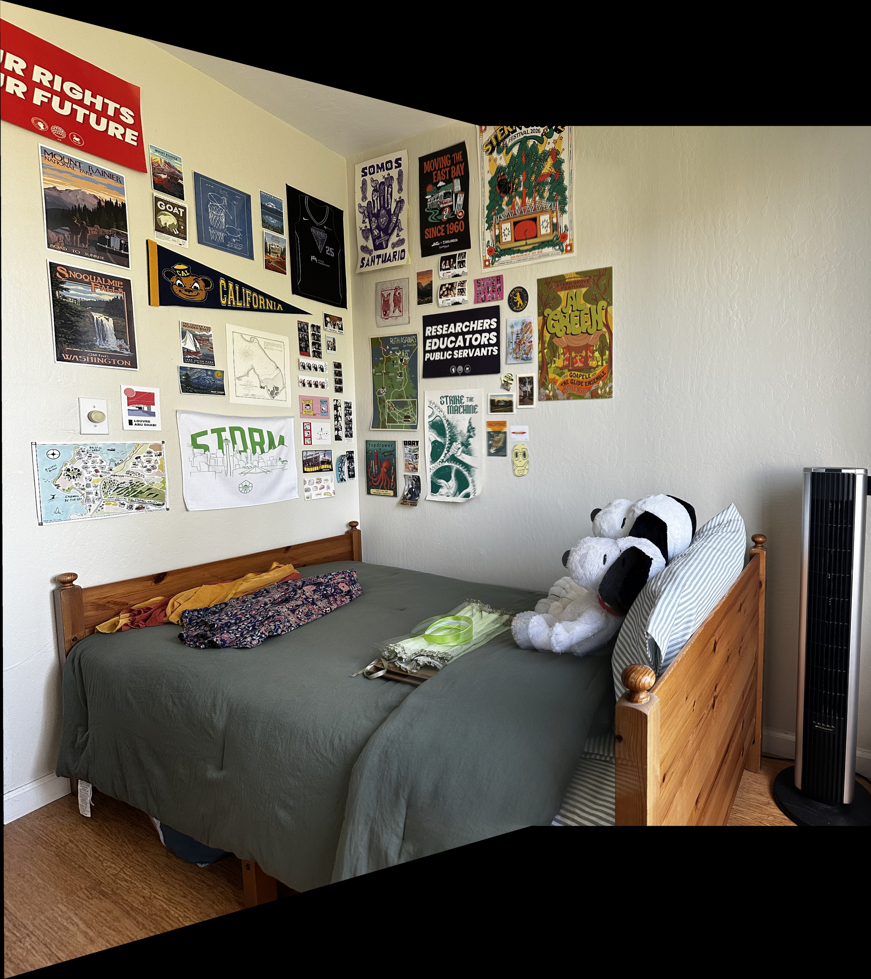
The wall posters align closely. The headband and stuffed animals have visible doubling, consistent with the depth differences that affected the original 12-point fit. Feathering softens the transition but cannot align those objects with the wall homography.
Kitchen Mosaic
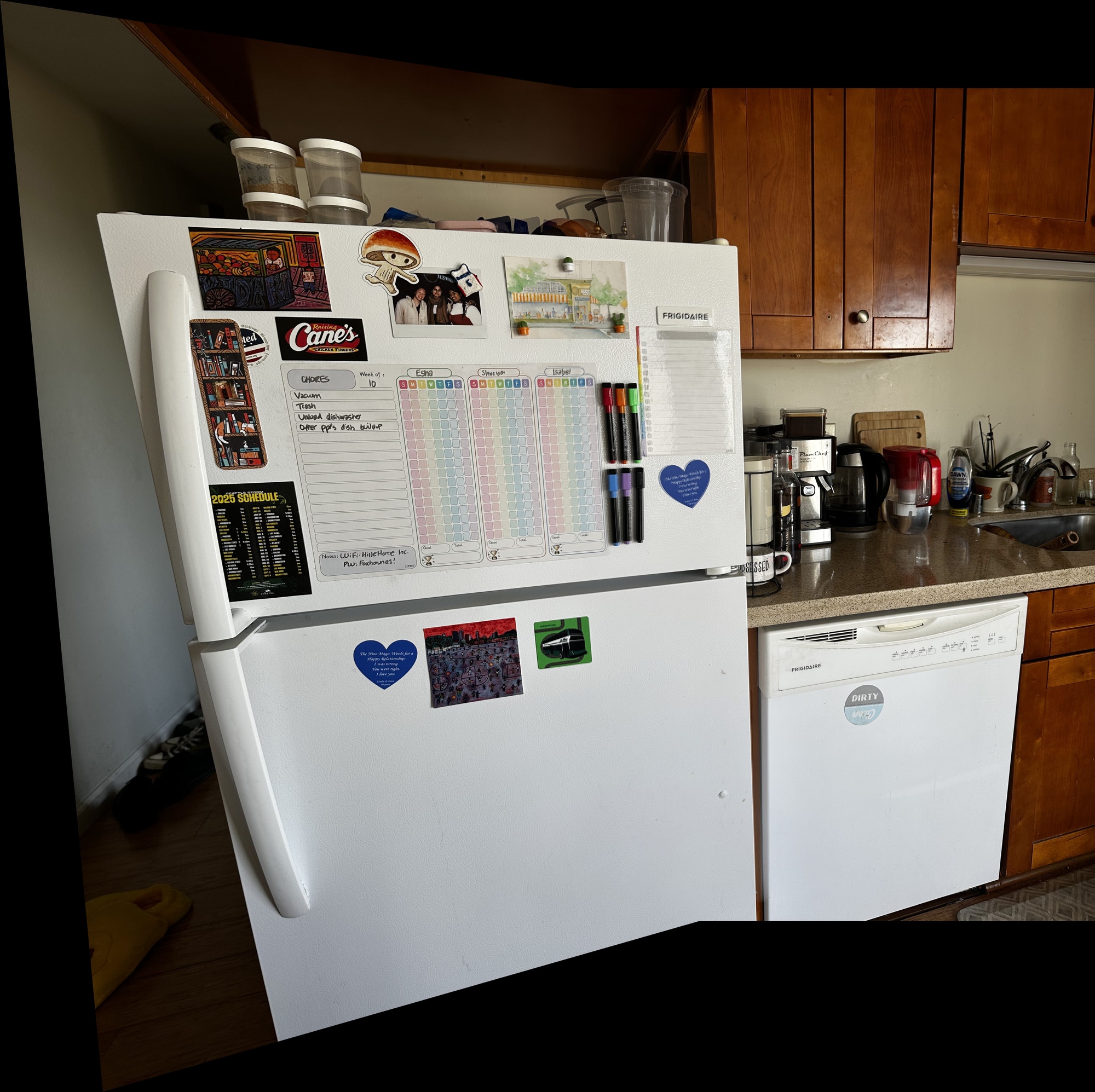
The fridge details align closely. The containers above the fridge show doubling, and there is a visible brightness difference near the cabinet transition. The homography was fitted to points on the fridge front.
Outdoors Mosaic
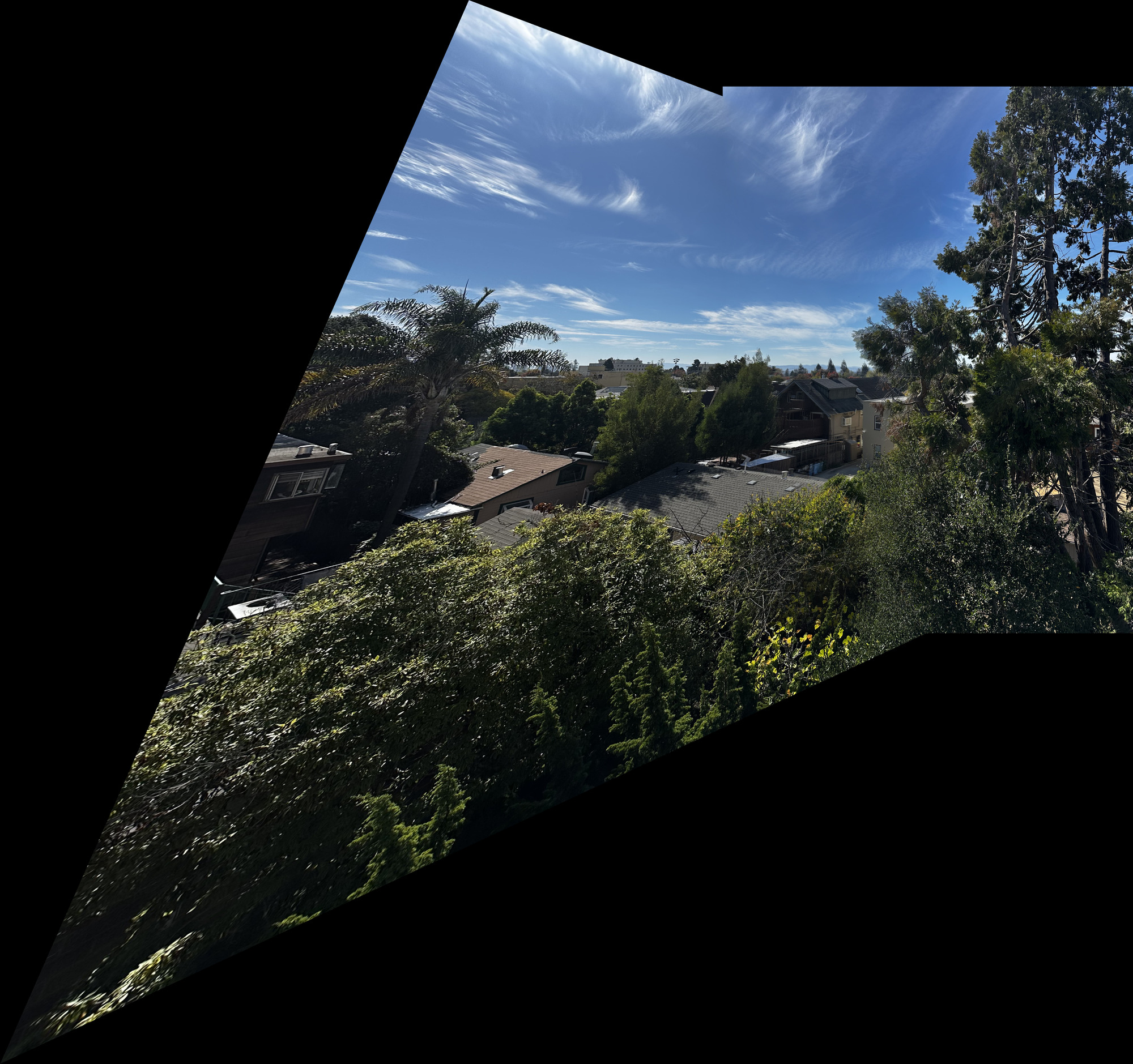
The buildings join reasonably at this display size, but the left side stretches strongly. The selected points occupy a small part of the overlap, so the low error at those points does not establish a good fit across the full image. Foreground trees also have a different depth from the buildings.
Part B: Feature Matching for Autostitching
In Part A, I clicked corresponding points by hand to tell the program which locations showed the same scene detail. In Part B, the program finds those correspondences automatically. It first chooses candidate points in each image, describes the appearance around each point, compares those descriptions across images, and uses RANSAC to select matches that agree on a homography. That homography then goes through the warping and blending code from Part A.
I used the same bedroom, kitchen, and outdoors image pairs. I resized each photo to 900 × 1200 pixels to reduce the cost of feature detection and matching.
B.1: Harris Corner Detection
A useful feature point has a recognizable neighborhood that can be found again in the other photo. Harris corner detection looks for locations where image intensity changes in two directions. Moving a small window across a flat wall changes little; moving along a straight edge can also change little. At a corner, movement in either direction changes the window’s appearance. This makes corners useful candidates for matching.
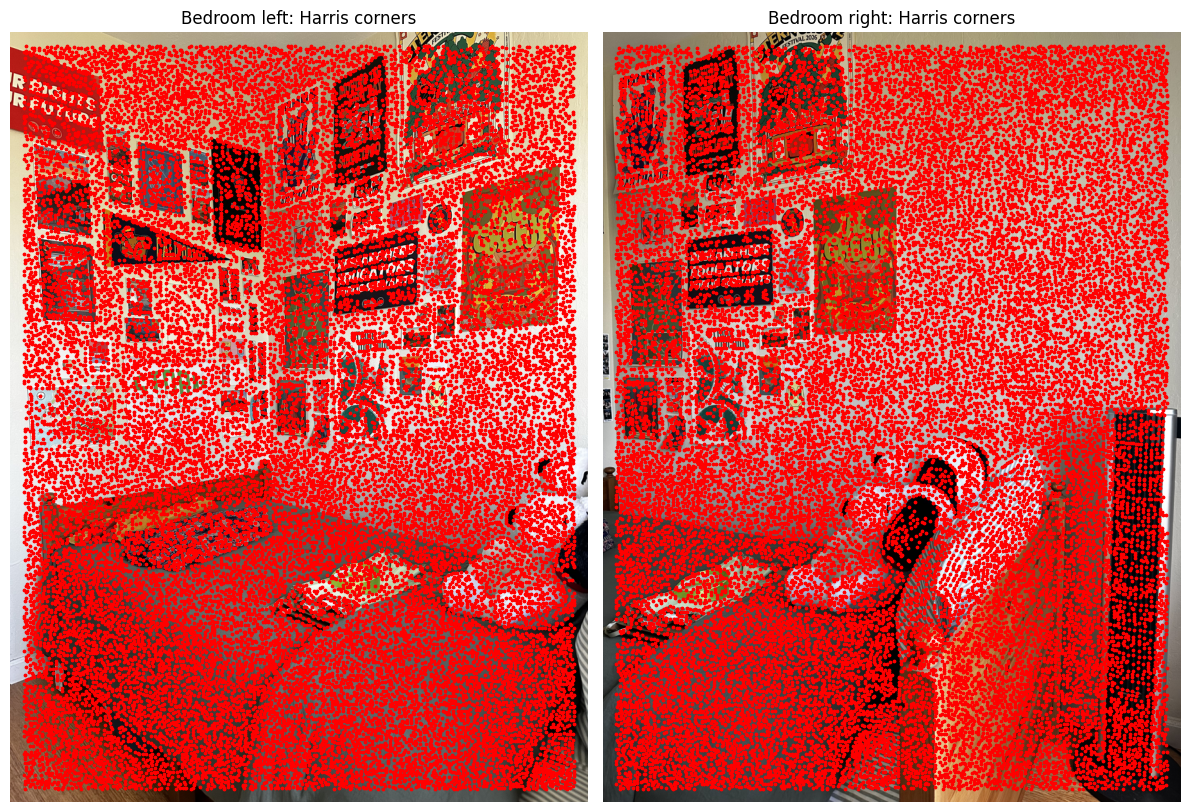
I used the supplied Harris detector at a single scale on grayscale images. It computes a corner response at each pixel, then returns local maxima and excludes points within 20 pixels of the image boundary. These are candidate locations only: detecting a point in the left image does not yet identify its partner in the right image. The red overlays below show that the initial detections are dense in textured areas.
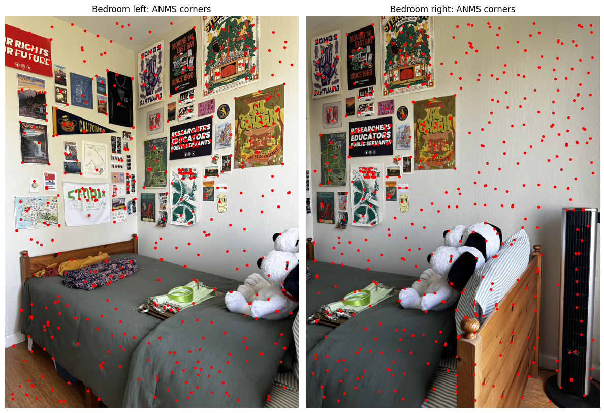
Keeping every candidate would make later matching expensive. Keeping only the strongest responses could also concentrate points in a few textured regions. Adaptive non-maximal suppression (ANMS) favors strong points that have some space around them, so the selected features cover more of the image.
For each corner i, I find the distance to the nearest corner j whose response satisfies fᵢ < 0.9fⱼ, where f is the Harris response. This distance is the corner’s suppression radius. A point close to a sufficiently stronger corner gets a small radius; an isolated strong point gets a large one. A point with no sufficiently stronger neighbor receives an infinite radius. I rank the radii and keep the largest 500 independently in each image.
The before-and-after plots show this reduction from roughly 25,000–27,000 candidates to 500 points per image.
| Scene | Left | Right |
|---|---|---|
| Bedroom | 26,780 | 26,605 |
| Kitchen | 26,888 | 27,082 |
| Outdoors | 25,507 | 25,176 |
Bedroom
Kitchen
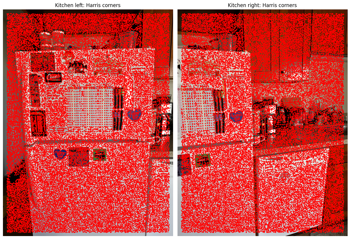
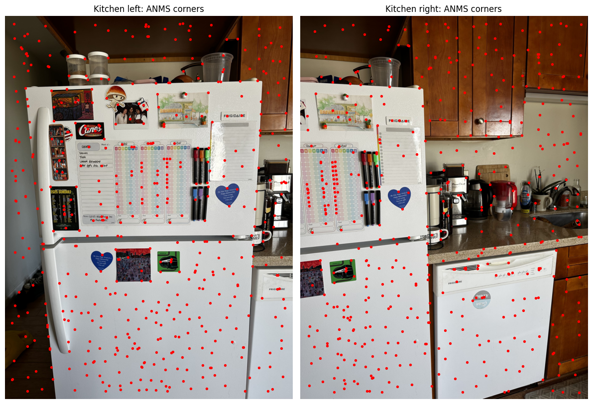
Outdoors
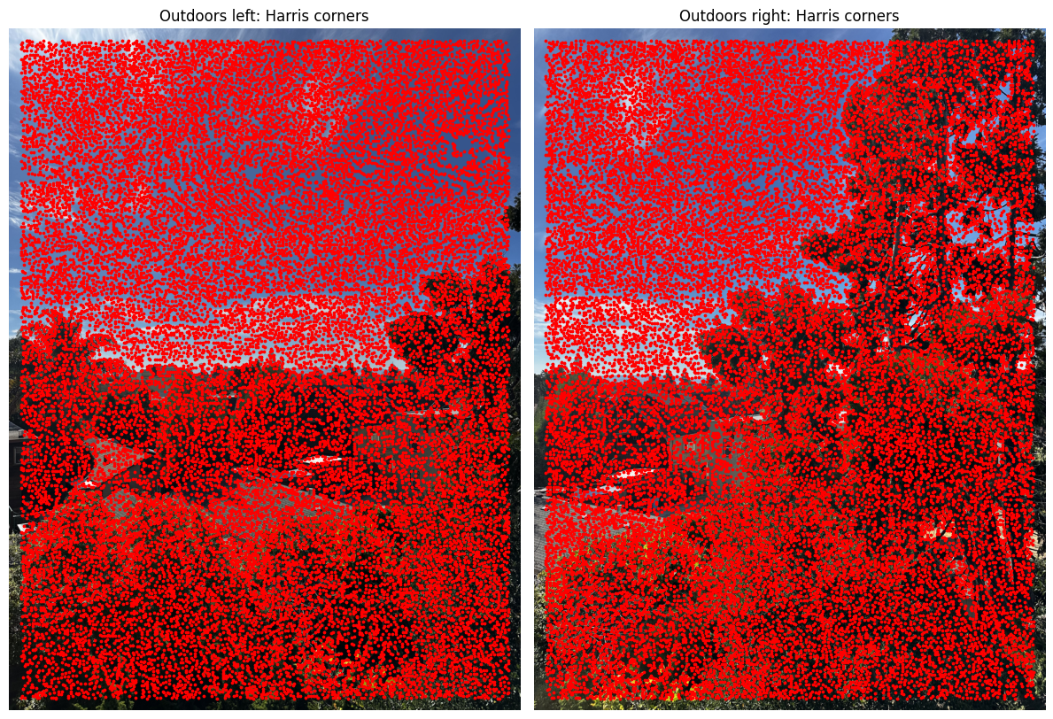
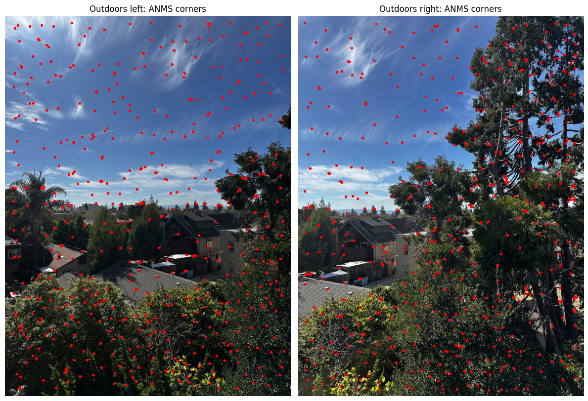
B.2: Feature Descriptor Extraction
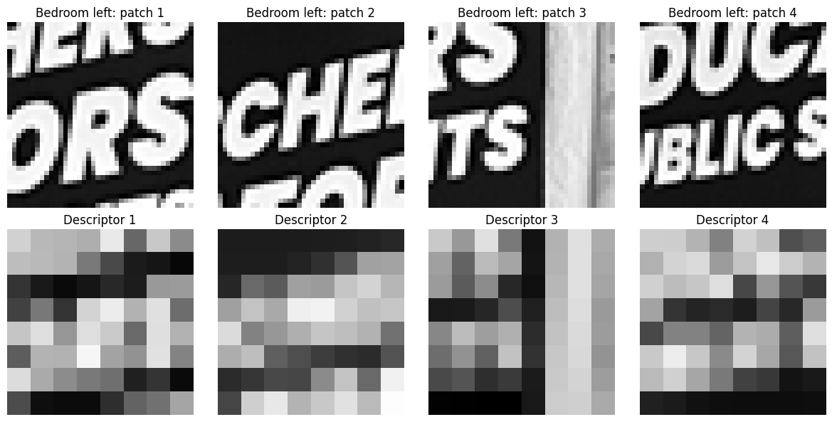
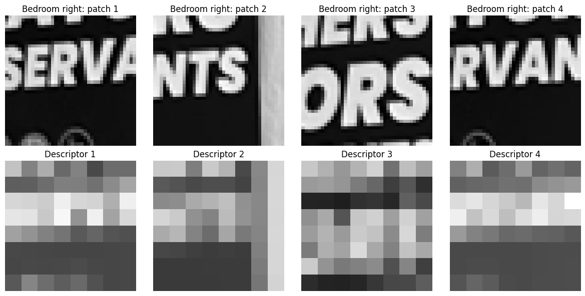
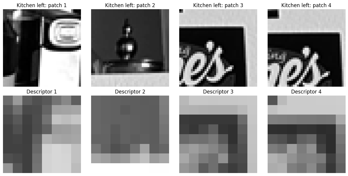
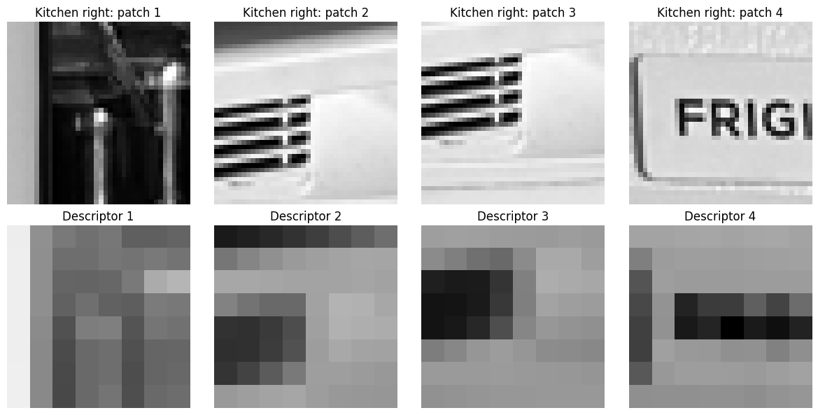
ANMS gives me point locations. To compare a point in one photo with points in the other, I also need a description of what surrounds it. A feature descriptor stores that local appearance as a small array of numbers. Points that show the same scene detail should have similar descriptors, even though their image coordinates differ.
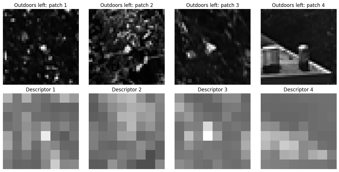
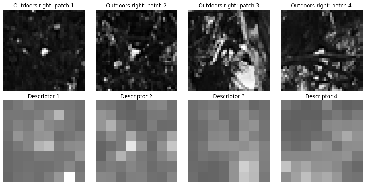
I blur each grayscale image with a Gaussian filter (σ = 2), then extract a 40 × 40 window around each selected corner. Sampling every fifth pixel near the center of each 5 × 5 block produces an axis-aligned 8 × 8 descriptor. The larger source window captures context around the corner; blurring before sampling reduces sensitivity to fine detail and small shifts. I keep the image axes fixed, so these descriptors do not compensate for rotation or changes in scale.
I flatten the 8 × 8 patch to 64 values, subtract its mean, and divide by its standard deviation. Subtracting the mean removes a uniform brightness offset. Dividing by the standard deviation adjusts the contrast scale. This helps corresponding patches compare well under simple brightness and contrast differences between photos.
descriptor = (sampled patch − mean) / standard deviationThe function skips windows that cross the image boundary and nearly constant patches, whose standard deviations are too small for reliable division. It keeps each descriptor paired with its point coordinates. All six images retained 500 descriptors, each with mean zero and standard deviation one.
Below, each top row shows four original 40 × 40 source windows; the bottom row shows their normalized 8 × 8 descriptors. Each column illustrates the conversion of one window into a descriptor.
Bedroom
Kitchen
Outdoors
B.3: Feature Matching
For each of the 500 descriptors in the left image, I compare its 64 values with every descriptor in the right image. I subtract corresponding values, square the differences, and sum them. This sum of squared differences (SSD) is small when two patches have similar normalized appearance. The right-image descriptor with the smallest SSD is the nearest neighbor.
A nearest neighbor alone can be misleading: repeated patterns can give several candidates with similar scores. I therefore compare the best match with the second-best match. I accept the best candidate only when its SSD divided by the second-best candidate’s SSD is less than 0.5.
ratio = SSD to best candidate / SSD to second-best candidate
accept when ratio < 0.5
For example, SSD values of 10 and 40 give a ratio of 0.25, so I keep the best match. Values of 10 and 12 give about 0.83, so I reject it: two candidates look almost equally plausible. A smaller ratio indicates a more distinct best candidate.
The threshold applies to squared distances, so it corresponds to about 0.707 for ordinary Euclidean distances. RANSAC then checks which matches agree with a single homography.
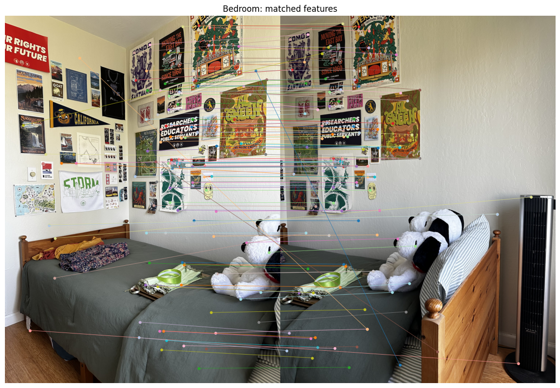
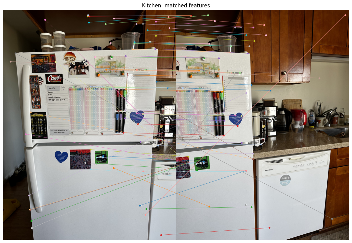
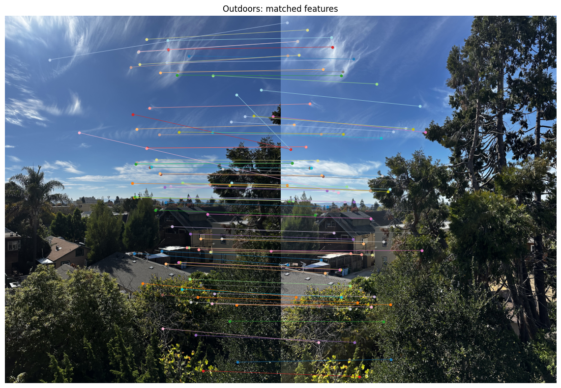
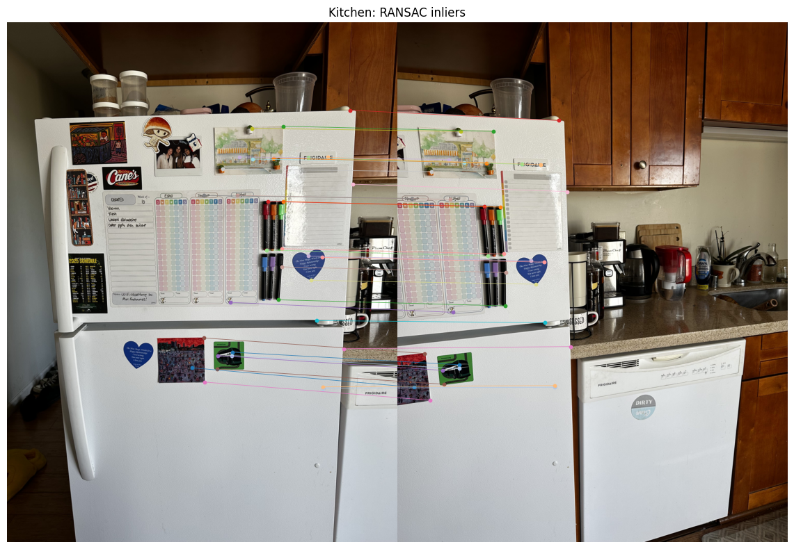
Each line in the plots below connects one accepted left-image point to its proposed right-image partner. The number of lines is smaller than 500 because many descriptors fail the ratio test.
| Scene | Matches |
|---|---|
| Bedroom | 122 |
| Kitchen | 76 |
| Outdoors | 86 |
Bedroom
Kitchen
Outdoors
B.4: RANSAC for Robust Homography
The ratio test gives proposed correspondences, including some incorrect ones. Fitting a homography to all of them at once could let those errors distort the result. RANSAC (Random Sample Consensus) searches for a homography that a large group of matches supports.
I implemented four-point RANSAC with 2,000 trials and a fixed random seed of 180. Each trial samples four matches without replacement and estimates a homography with computeH. Four point pairs provide the eight equations needed for the eight unknown homography entries, provided the points form a suitable configuration. The implementation skips samples with repeated destination points and estimates that are invalid or singular.
I test each candidate homography against every proposed match. I project the left-image point into the right image and measure the Euclidean distance to its matched right-image point. A match with an error below 3 pixels is an inlier for that candidate. The other matches are outliers for that candidate.
predicted right point = H · left point, divided by its homogeneous coordinate
error = distance(predicted right point, matched right point)
inlier when error < 3 pixels
I keep the candidate with the largest inlier set. I then refit the homography using all matches in that set, which gives an overdetermined least-squares fit as in Part A, and recompute the inlier mask with the fitted homography. Repeating the random trials gives the algorithm chances to draw four consistent matches despite the outliers.
The table reports the final inlier counts and their mean projection errors after refitting. For example, the bedroom result retains 80 of the 122 proposed matches.
| Scene | Matches | Inliers | Mean Inlier Error |
|---|---|---|---|
| Bedroom | 122 | 80 | 1.27 px |
| Kitchen | 76 | 33 | 1.26 px |
| Outdoors | 86 | 45 | 1.42 px |
I pass the estimated homography to stitch_images, which reuses Part A’s bilinear warping, shared canvas, and distance-weighted blending. It warps the left photo into the right photo’s coordinates, places both images on a canvas large enough to contain them, and blends their overlap. The automatic part is the selection of correspondences and estimation of the homography.
For each comparison below, the manual mosaic uses the clicked points from Part A, and the automatic mosaic uses the feature matches selected by RANSAC. Both use the same resized photos and blending code. I convert each original-resolution manual homography to the resized coordinate system with H_small = S H_original S⁻¹, where S scales pixel coordinates. This maps a resized source point back to original coordinates, applies the original homography, then scales the destination point down again.
Bedroom
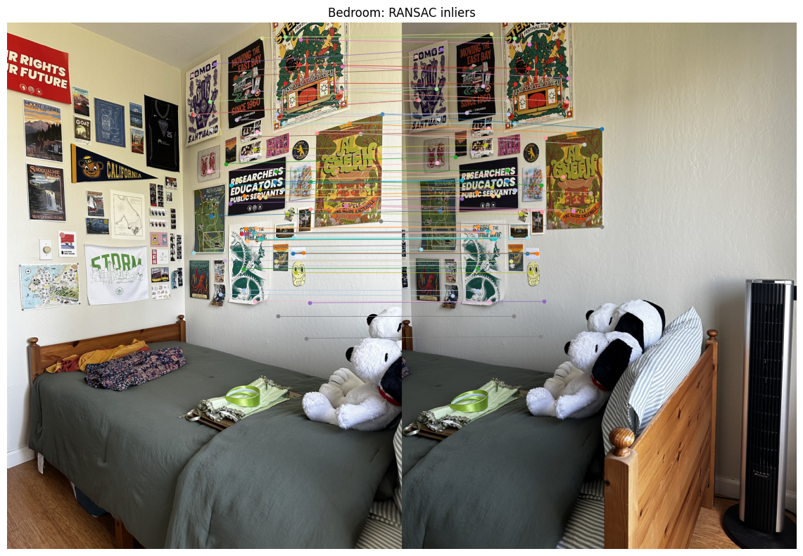
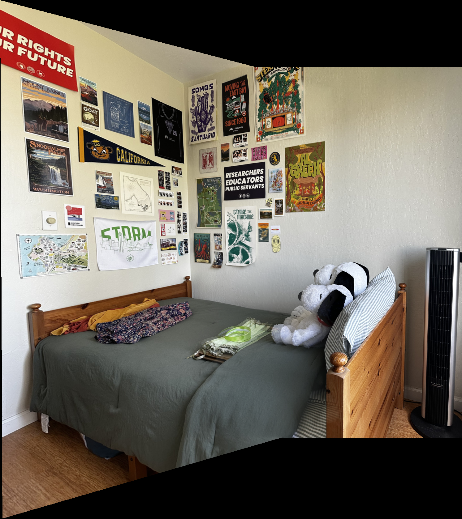
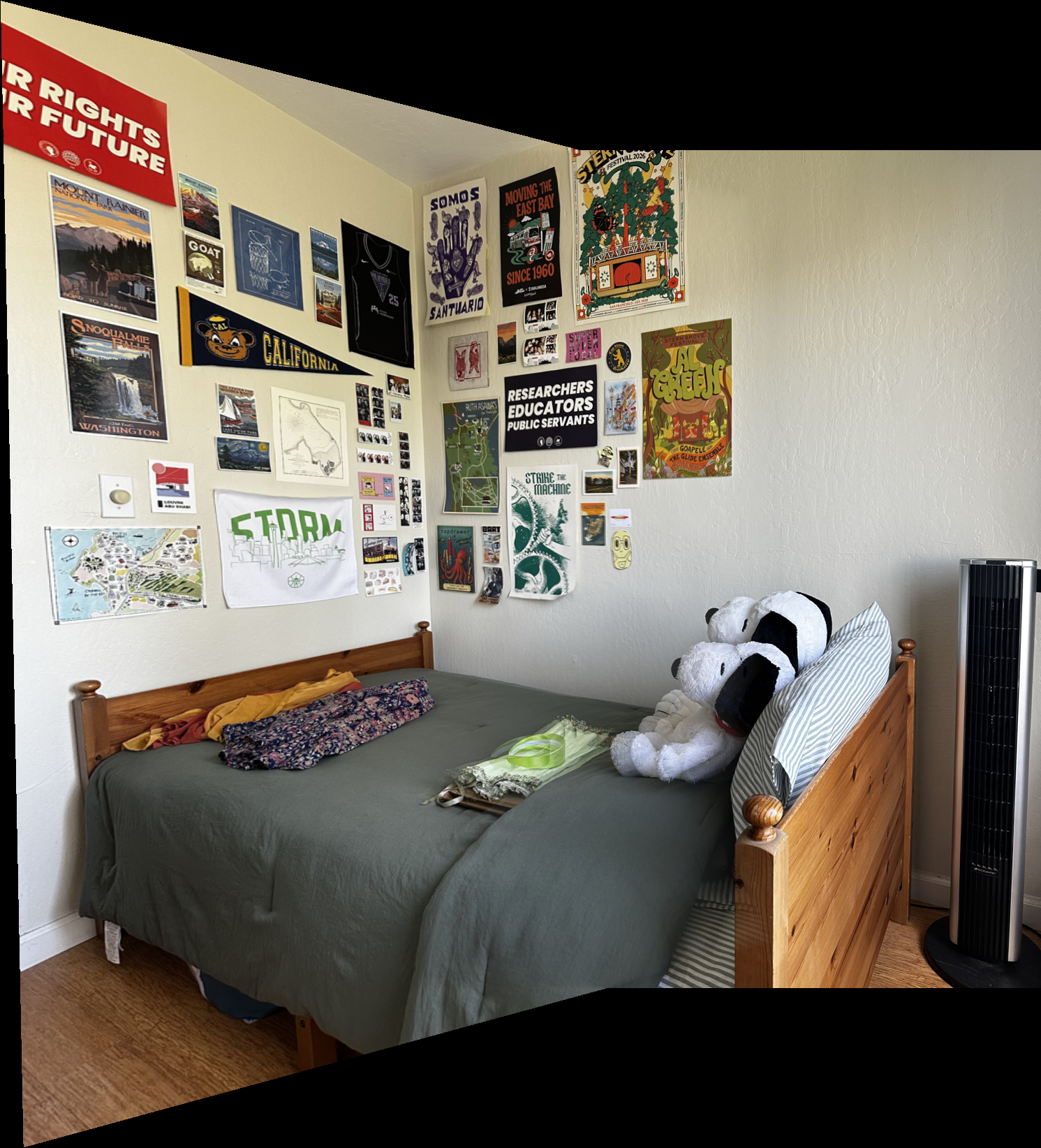
The wall posters align closely in both mosaics. The headband and stuffed animals still show doubling because the nearer objects and the wall have different depths.
Kitchen
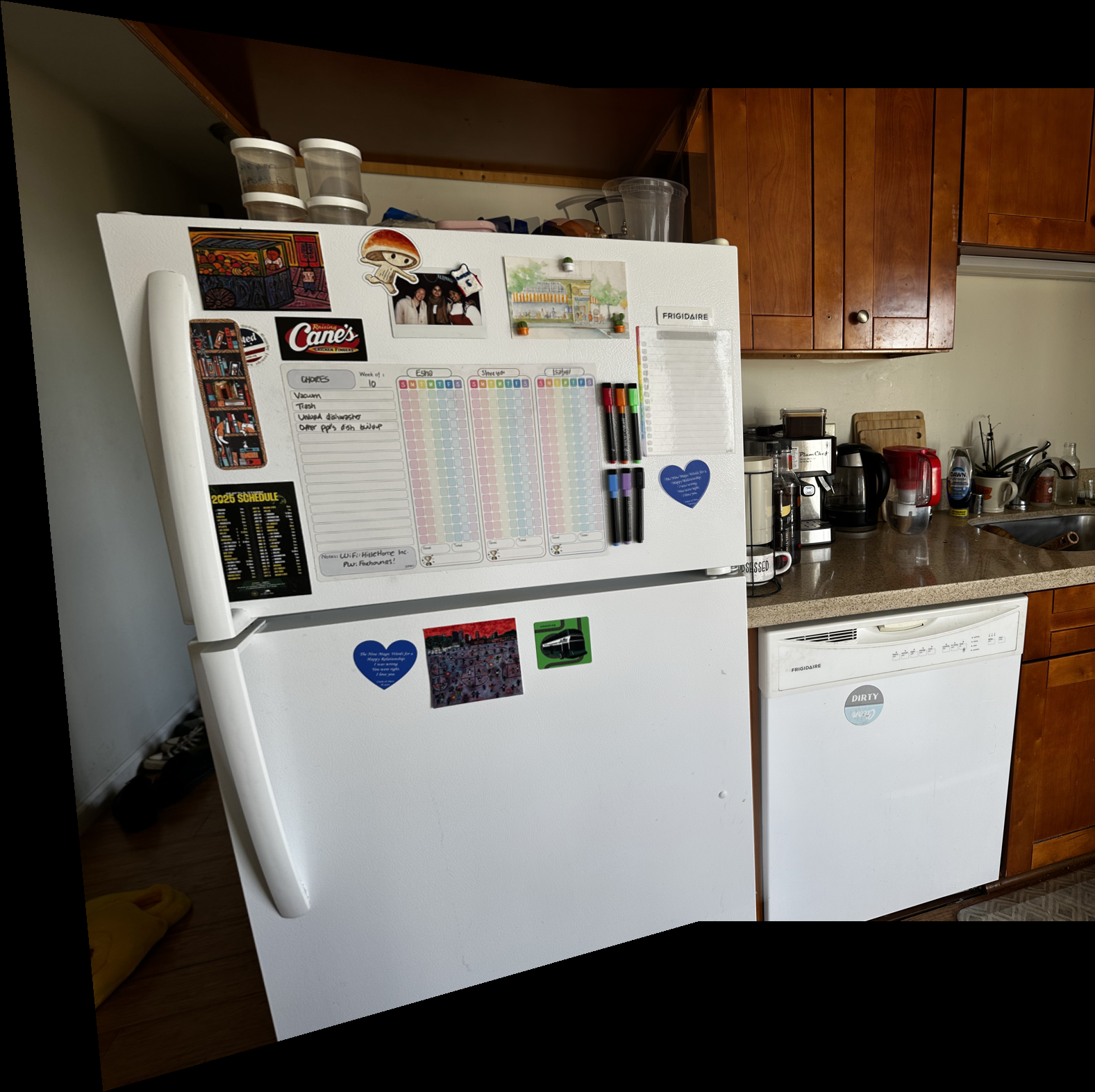
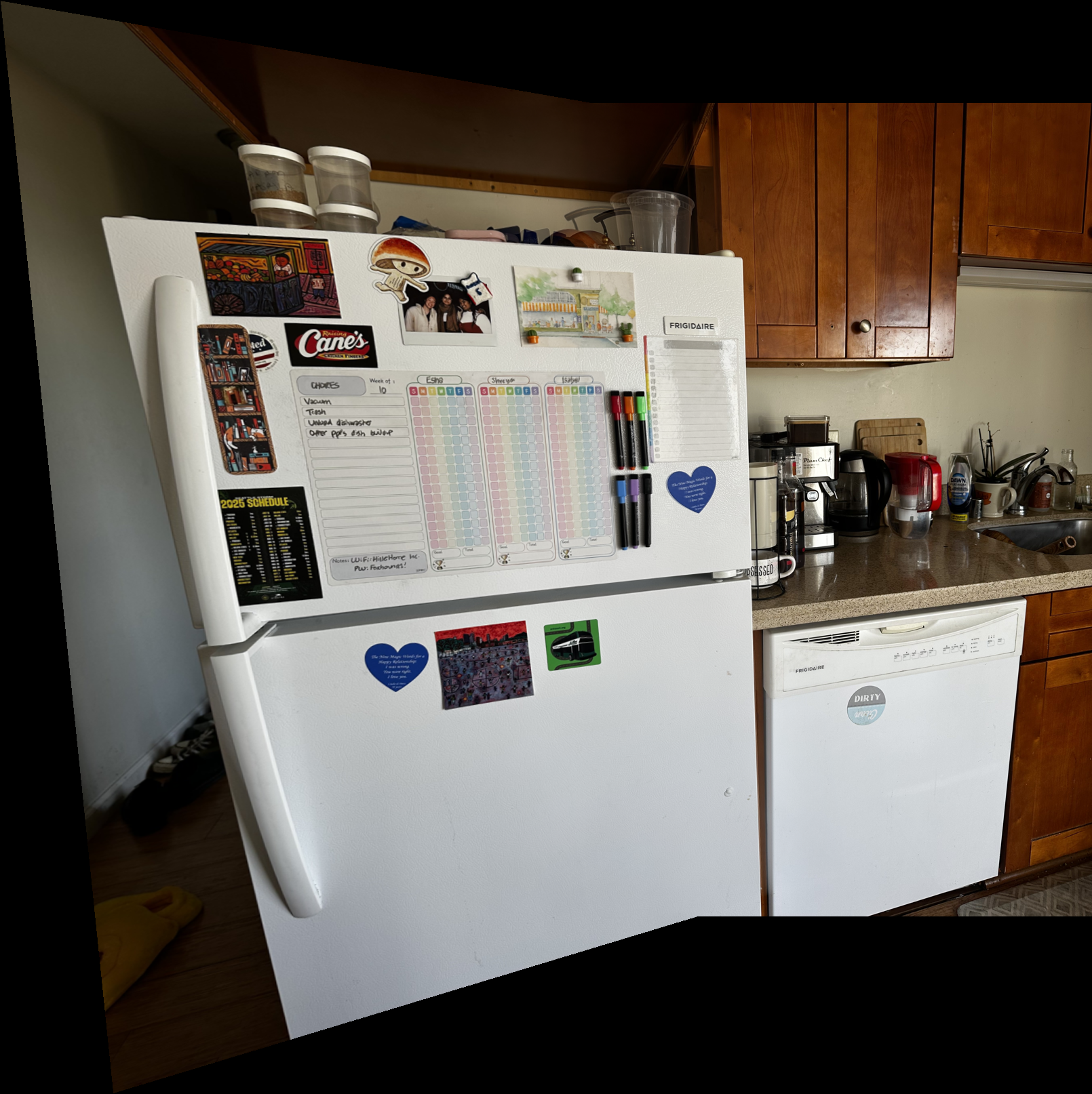
The fridge details align closely in both results. The containers above the fridge still show doubling, and a brightness difference remains near the cabinet transition.
Outdoors
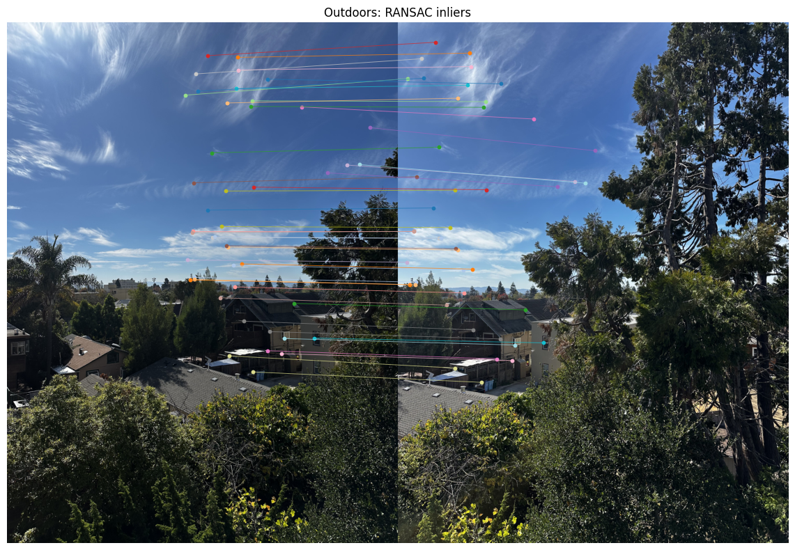
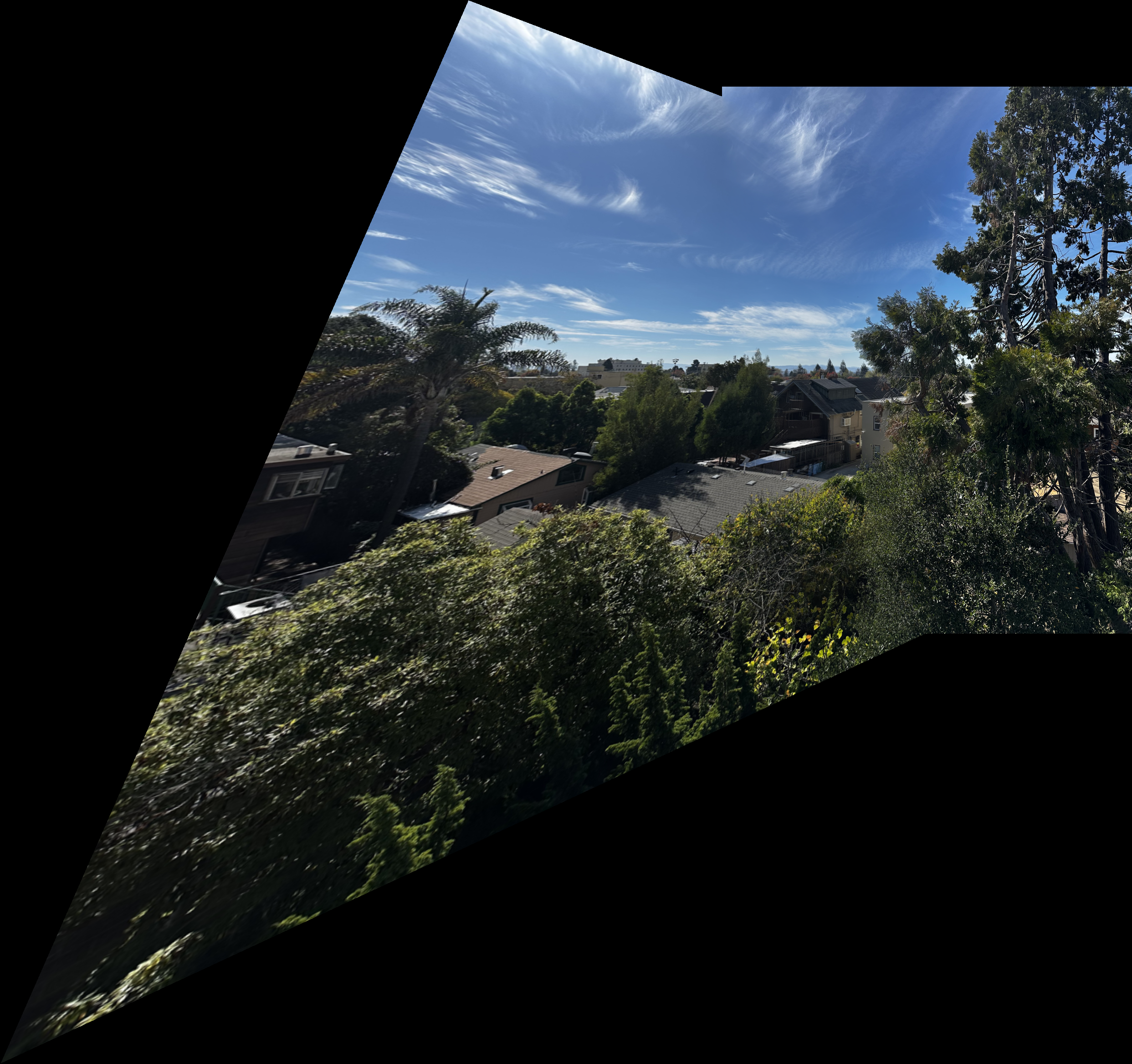
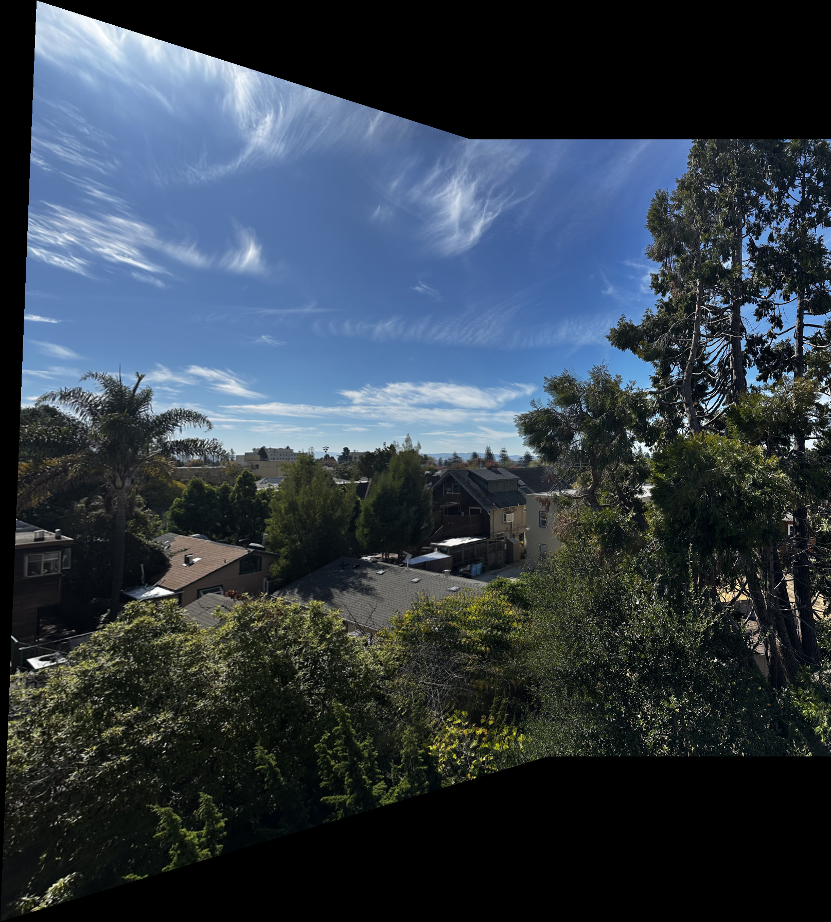
The automatic result has much less stretching on the left than the manual result. The automatic matches cover more of the scene than the eight manually selected building points. Foreground trees can still show misalignment because of depth differences.